
|
Chloride and Heavy Metals in HCC’s Stream Systems Stephen Shaner, Howard Community College Mentored by: Hannah Pie, Ph.D. and Rebecca Carmody, Ph.D. |
Abstract
Stream pollution caused by road runoff is a problem for stream ecosystems and the overall quality of the water. Many different pollutants accumulate on roads and can be washed into streams by storm runoff, such as trash, road salts, and metals. Our goal for this project was to monitor the levels of manganese, iron, nickel, and chloride in two streams on the Howard Community College (HCC) campus in order to monitor how the overall health of the streams may be affected by road and construction site runoff. We collected monthly water samples from five locations on two campus stream systems. We examined the water quality at each site using sensors and then analyzed the concentrations of manganese, iron, and nickel using an atomic absorption spectrophotometer. Iron and manganese levels varied by location with one site (Site B) consistently having the highest concentrations of both metals. However, nickel was generally below the detection limit in most of the sites, besides notably the closest site to the ongoing campus construction project (Site D). Another notable aspect of the data is that in 2023 there was an overall decrease in average chloride concentrations across all sample locations for the year which could be related to a decrease in road salt application during the winter of 2022-2023 due to the almost complete lack of snow. In the future, we hope to look closer into microbial growth in Site B that could influence the levels of manganese and iron at that location, as well as determine if some of the rocks at Site B that were seemingly placed to reduce erosion at the outflow of the culvert have any effect on the iron and manganese concentrations at the site.
Introduction
Stream pollution is an all-too-common problem which can be caused by many different things. Common sources of pollutants are construction and roads [1]. Runoff from roads commonly contributes to stream pollution in the form of heavy metals and road salts [2]. Over the past few decades, there has been increasing awareness of and research carried out on the contribution of road salt to stream pollution [2,3,4]. Undesirable effects of the increased salinization of freshwater streams includes decreased biodiversity of aquatic life forms in the stream [5] and stream water exceeding the EPA recommendation for chloride in drinking water [6]. Increased chloride (Cl-) in stream water and in the ground water feeding streams, in turn, can produce a cascade of other effects, including releasing metals adsorbed to soil particles [2].
Heavy metals and chloride are a concern for the ecosystems and aquatic food webs of freshwater stream environments, and it has been well documented that streams near roads are especially impacted [2,4]. While some heavy metals have high toxicity at lower concentrations, other heavy metals like iron (Fe), manganese (Mn), and nickel (Ni) are required by organisms for certain biological processes and typically have lower ecological toxicity at concentrations normally measured in most environments [7,8,9]. Chloride also can be toxic to freshwater aquatic organisms at higher concentrations [2,3].
Iron is an essential nutrient for many organisms; however, it can be potentially toxic in high concentrations [8,10,11]. The EPA lists the chronic aquatic life limit for Fe in freshwater as 1000 μg/L [12]. (Aquatic Life Limits and Secondary Drinking Water Standards are discussed in more detail in the Results section.) Manganese is also usually considered a non-toxic metal, however more recent research has found that in higher concentrations it can be toxic to mammals, such as humans, causing Parkinsons-like symptoms [7]. The secondary maximum contaminant level (SMCL) established by the EPA for Mn in drinking water is listed as 50 μg/L for aesthetic reasons not related to toxicity [13]. Nickel is also considered generally safe and non-toxic unless it is found in substantial concentrations. The EPA lists the chronic aquatic life limit for Ni in freshwater as 52 μg/L [12]. Cars are a major source for certain metals that accumulate in roadside soils, with metals such as Ni being released by brake and tire wear as well as vehicular degradation, i.e., rusting [2, 14]. Industrial processes are also a common source of Ni pollution in the aquatic environment [14]. While there are many possible ways for metals such as Fe and Mn to enter streams and groundwater, mobilization (or movement from soil, sediment, or rock into water) of these metals under saline (salty) conditions is an important effect [2, 3, 15]. In addition, Kaushal et al. [15] have stressed the need for additional studies monitoring the effect of Cl- concentrations on mobilization of metals in freshwater ecosystems, particularly those in more humid environments like what is experienced in Maryland.
Chloride levels in many stream systems are on the rise [15] because of an increase in the application of road deicing salts over the years [3]. This increase in road salt usage is a problem because road salt does find its way into surface freshwater sources and can be toxic to animals and plants, which alongside the previously mentioned mobilization of metals is potentially even more toxic than the road salts on their own [2]. These road salts can also make their way into groundwater and other drinking water sources [15]. Additionally, the EPA’s freshwater chronic (long-term exposure effects) aquatic life criteria limit is 230 mg/L and their acute (short-term exposure effects) aquatic life criteria limit is 860 mg/L for chloride [12]. Dugan et al. predicted in 2017 that if the then-current rate of salinization of lakes in the north-central and northeastern US continued unchanged, that of the 284 lakes they studied, 47 would exceed 100 mg/L Cl- by 2050 and 14 of these would exceed the EPA’s chronic aquatic life limit of 230 mg/L Cl- by that year as well [16].
The motivation for the current study was to investigate the extent to which excessive chloride and metals might be an issue affecting the stream systems on the Howard Community College (HCC) campus. The main goal of our study was to monitor the concentrations of heavy metals (Mn, Fe, and Ni) and Cl-, and other water-quality parameters in two stream systems on campus, to compare these levels to water quality limits, to compare values measured in 2023 to data from past studies on campus, to examine correlations between parameters, and to document the possible impacts of the Math-Athletic Complex construction process on its closest stream system.
Methods
Preparation of materials
The high-density polyethylene bottles used to collect samples and all other processing glassware or plasticware were all washed with lab detergent and tap water, then rinsed three times with deionized (DI) water. The resistivity of the DI water used was greater than 2 megaohms, indicating high purity. After this process they were soaked in 4% w/v nitric acid (HNO3), and then rinsed three more times with deionized water. The 4% w/v HNO3 was prepared from trace metal grade 70% w/w HNO3 and DI water. The collection bottles and processing equipment were then oven-dried at 50º C. The process for choosing and preparing the sampling containers used in this study was based on methods described in Standard Methods for the examination of Water and Wastewater [17] and Milivojevic et al. [18] and Varol and Şen [19]. The purpose was to eliminate impurities and metals which may be inside of the containers before they were used to collect and store samples.
Sample collection
Water samples were collected monthly in 2023 from 5 sites around the HCC campus located on two stream systems (Figure 1). Sites A, B, and B’ are situated in a wooded area on campus close to a busy road. Site B’ is not part of the steam, but a separate culvert which flows into Site B. This culvert has a continuous flow into Site B throughout the entire year. This water was tested to see what is flowing into B from this outside source compared to what comes from upstream. Site C and D are a part of a separate stream system on the other side of campus. Site C is a large pond and the water was collected towards the edge. Site D is the stream outflow from three culverts which run underneath Campus Drive, and trash was frequently seen in the Site D sampling location just downstream from these culverts. The stream flows from Site D into the pond. Sites C and D are also notably very close to the recent construction on campus.
At each sampling location, water samples were collected at a depth of 10 cm. Two separate polyethylene bottles of water were collected at each location: a 1 L bottle for metal analysis and a 250 mL bottle for water quality analysis. Polyethylene bottles were selected to minimize leaching of metals from the storage containers [20]. All water samples were collected while wearing gloves and while the bottle was fully submerged under the water to avoid any possible contamination by air or surface water/materials. Water samples for metal analysis were placed on ice for preservation until processing.
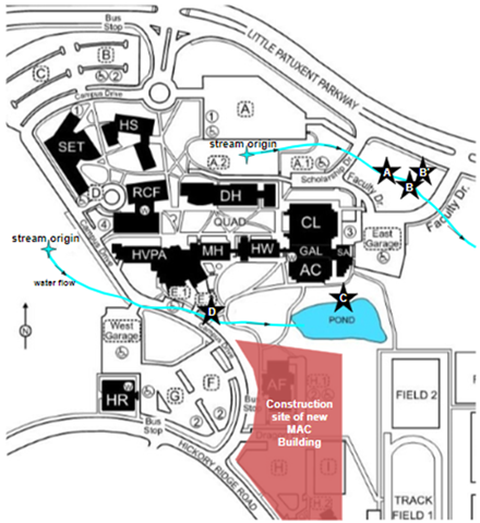
Figure 1: HCC Campus map with the location of the five sampling sites (A, B, B’, C, and D) along the two stream systems and the pond. The location of the MAC construction site is also included.
Sample processing
Each water sample was further processed within the lab by filtering through a 0.45 μm MF-Millipore nitrocellulose membrane filter by vacuum filtration into a clean acid-washed 1 L polyethene flask and then poured into a second clean, acid-washed polyethylene bottle in order to avoid impurities that could affect our measurement of dissolved metals. Before the sample was filtered, 100 mL of 2% w/v HNO3 made from trace-metal grade 70% w/w HNO3 was run through the filtering apparatus in order to wash the filter and to detect any possible contamination that persisted through the cleaning process [17]. This filter blank was stored in an acid-washed 250 mL polyethylene bottle at 4°C for later metal analysis. After the filter blank was taken, the water sample was filtered. If the filtration slowed down to a point where it was difficult to filter efficiently, then a new filter was used. After the new filter was applied, 50 mL of 2% w/v HNO3 was run through it but was disposed of and not collected. A different clean set of equipment was used for each sample to prevent any potential cross-contamination between samples from different sites.
After filtering was complete the samples were acidified to a pH of 1 using trace-metal grade 70% w/w HNO3 [17]. The samples were inverted a few times to distribute the HNO3 equally throughout and the samples were then refrigerated until further analysis.
Water quality testing
During the water sample collection process, measurements of both air and water temperature, barometric pressure, and dissolved oxygen were obtained at Sites A, B, C, and D using Vernier sensors. The water depth at each sampling location was also measured using a clean ruler.
Using the water samples in the 250 mL bottles, additional water quality parameters were measured in the lab within one to two hours of sample collection. Chloride, pH, conductivity, and turbidity were measured using Vernier sensors that were each calibrated using a two-point calibration method. Turbidity is a measure of the opaqueness or cloudiness of water. It is measured with a sensor that shines light through the sample and measures how much of the light passes through the sample versus how much light is scattered [17]. Calibration curve voltages for each sensor were recorded each day of sampling and compared across the year to ensure validity. Additionally, nitrate and phosphate levels were measured using test kits following each kit’s protocol. The nitrate kit (API) had color card identification measurement ranges of 0, 5, 10, 20, 40, 80, and 160 mg/L. The phosphate kit (Natural Chemistry) had color identification measurement ranges of 0, 100, 200, 300, 500, 1000, and 1500 μg/L.
Heavy metal analysis
The water samples and filter blanks were analyzed using a Shimadzu AA-7000 atomic absorption spectrophotometer (AAS) in graphite furnace mode using a pyrolytic graphite tube and either a manganese or a nickel/iron hollow-cathode lamp. A small amount of sample is introduced to the graphite tube in the AAS, which is then vaporized and light of a specific wavelength is shown through it. The instrument detects the amount of light transmitted through each sample. The software that runs the AAS reports the absorbance of the sample. Each metal had a specific wavelength of light which worked best for measuring it; these are 279.5 nm for Mn, 248.3 nm for Fe, and 232.0 nm for Ni [17,21]. According to Beer’s Law [22], the absorbance of light is directly proportional to the concentration of the metal in the solution, so we used the absorbance of light measured to quantify the concentration of each metal in our water samples. In order to do that, a standard calibration curve for each metal was created by plotting the measured absorbances on a series of solutions of known concentrations of that metal. From this plot, a linear regression trendline (y=mx+b) was added and used to directly compare absorbance (y) to concentration of metal (x). Each trendline’s reliability was examined using its R2 value with all values greater than 0.98. The solutions of known concentration (standards) for each metal were prepared by a series of dilutions from a stock (1000 mg/L) solution for each metal (Inorganic Ventures). The lowest known concentration measured for each metal was treated as the detection limit for that metal. The detection limits were 0.5 μg/L for Mn, either 4 or 5 μg/L for Fe (depending on each graphite tube’s sensitivity), and 0.75 μg/L for Ni. Using the trendline for each metal, we calculated the concentration of the metal of interest in each water sample from its measured absorbance.
The water samples for Ni could be measured directly as all concentrations were below the highest calibration curve concentration. However, the concentrations of Mn and Fe in many of the water samples were above the concentration in the highest calibration standards and needed to be diluted before being analyzed in order to get an absorbance within the calibrated range. When measuring Mn and Fe, water samples were diluted by different amounts ranging from 2 -100x dilution factors depending on the starting concentration. All dilutions were made using 2% w/v HNO3 made using trace-metal grade 70% w/w HNO3. All water samples were analyzed three to four times depending on the reproducibility of the first three measurements, and the three measurements with the best precision were averaged and both a standard deviation and standard error were calculated. To ensure reproducibility across the year and accuracy of some of the more heavily diluted samples, some samples were measured multiple times and an average concentration was calculated for these duplicate runs. Due to the high concentrations of Mn and Fe in some water samples, even with dilution, an aliquot of 2% w/v HNO3 was measured three to four times between each water sample to ensure there was no carry-over when measuring the next water sample. This was not needed when measuring Ni since Ni concentrations in the water samples were much lower.
Statistical Analysis
Spearman’s rank correlation analyses were conducted to compare between metrics (chloride concentrations, conductivity levels, Fe concentrations, and Mn concentrations) using R software. Relationships were examined between chloride and conductivity as ions like chloride influence the overall Conductivity (or resistivity) of a solution. Relationships were examined between chloride, Fe, and Mn as chloride has been shown to cause the mobilization of both metals in aquatic environments [2, 3, 15]. No other metrics measured showed visual relationships of interest, so correlation analyzes were not performed for them. This type of rank correlation analysis was performed because not all metrics displayed a normal distribution. A p <0.05 was used to determine if the correlations were statistically significant. The rho values representing the strength of each correlation were calculated for each analysis. The closer rho is to either 1 or -1, the stronger the positive or negative correlation, respectively. Some correlations were conducted using the year’s data for all five sites, while others were conducted by comparing the year’s data at only Sites B and/or B’.
Results
Precipitation considerations
Concentrations of metals, chloride, and water quality parameters of samples collected were influenced by higher amounts of precipitation during three months: April, July, and December. The actual sample collection on 4/28/23 occurred during a heavy rain storm. While there was no direct precipitation during sampling events on 7/20/23 and 12/21/23, both months had higher-than-average precipitation levels. Rainfall for the following months in 2023 were below normal: January, February, March, May, June, August, October, and November. Total rainfall in April 2023 was above normal with 1.34 inches (”) falling on the collection date of 4/28/23. From July 1 to 20, 2023, a total of 3.62” of rain fell at BWI Airport – this is 0.82” more than normal for this point in July. Also of note is that there was a thunderstorm in the early morning hours of July 19, which was the day before samples were taken. This thunderstorm produced 0.75” of rain. There was 5.48 inches of rain that fell at (BWI airport) between December 1-19, 2023; this is 3.23 inches more than the normal amount of rain for this point in December. The rain that fell during these months served to dilute the streamwater and thus led to lower measured concentrations of metals and chloride in most of the samples.
Water quality results
Multiple common metrics of stream water quality (pH, conductivity, dissolved oxygen, turbidity, nitrate concentrations and phosphate concentrations) were measured in this study. Table 1 shows yearly ranges and averages of pH, conductivity, dissolved oxygen, and turbidity at all sampling locations. The data for nitrate and phosphate concentrations is not shown in a table. Here we summarize the monthly trends and specific values of note.
The pH values across all sampling locations were relatively consistent throughout the year ranging from 6.5 – 7.8. The average and standard deviation for pH across all sites and months of 7.1 +/- 0.3.
Conductivity was highly variable throughout the year for all sampling locations, with Site C having the lowest variability. With the exception of Site C, the conductivity at all other sampling locations had their lowest measured value during the heavy rain sampling event in April, which was substantially lower than the month preceding it and the subsequent month. Additionally, the conductivity at all locations except Site C was lower than preceding months for July and December, both of which had extensive total precipitation. The dilution effect caused by individual rain events was much less pronounced in the case of Site C (the pond) due to its much larger volume.
At Sites A and B, dissolved oxygen (%) was lowest in the Spring and Fall (May – November) when there was a lot of leaf/plant debris or microbial growth observed in the streams. Site D was more consistent in its dissolved oxygen than other sampling locations, but the levels observed were slightly lower in the warmer months of April – August. Site C, however, had the opposite relationship with the highest dissolved oxygen in warmest months (May – August) with all these months displaying levels greater than 100%. Dissolved oxygen was not measured in water samples from the culvert (Site B’).
Turbidity was generally low in Sites A, B, and B’ throughout the year with all but one month at each site (April for B and B’ and June for A) being below 10 NTU (nephelometric turbidity unit). While most months for Sites C and D had comparatively low turbidity levels, both of these sites had three months each with levels elevated above 20 NTU. For Site C, these were the samples collected in July, August, and December with values of 30.3, 20.3, and 35.2 NTU, respectively. For Site D, these were the samples collected in July, September, and November with values of 163.5, 20.7, and 38.8 NTU, respectively.
Nitrate and phosphate levels were measured each month in Sites B and D as proxies for each stream system (data not shown) to examine the extent of excess nutrients in the stream systems. Nitrate concentrations ranged from 5 – 10 mg/L throughout the year at both sites with the exception of one month each that was measured at 20 mg/L. This was on 6/29/23 for Site B and 3/31/23 for Site D. Phosphate concentrations ranged from 0 – 100 μg/L throughout the year at both sites. Only nitrate concentrations above 10 mg/L are of concern to the health of the stream system [23] and all phosphate concentrations were below levels of concern for stream health [24]. More detailed water quality data is available in a supplement below.
|
pH
|
Conductivity (μS/cm) |
Dissolved Oxygen (%) |
Turbidity (NTU) |
|||||
| lowest – highest | average +/- stdev | lowest – highest | average +/- stdev | lowest – highest | average +/- stdev | lowest – highest | average +/- stdev | |
| Site A | 6.7 – 7.8 | 7.0 +/- 0.3 | 74 -1794 | 1187 +/- 562 | 63.2 – 96.5 | 82.0 +/- 13.2 | 0.0 – 12.6 | 3.3 +/-3.7 |
| Site B | 6.5 – 7.8 | 7.0 +/- 0.4 | 96 – 1684 | 1273 +/- 477 | 58.7 – 104.2 | 83.8 +/- 15.4 | 0.4 – 13.9 | 5.4 +/- 4.0 |
| Site B’ | 6.5 – 7.8 | 7.1 +/- 0.3 | 94 -1507 | 1286 +/- 381 | N/A | N/A | 0 – 16.3 | 4.4 +/- 4.8 |
| Site C | 6.7 – 7.7 | 7.2 +/- 0.3 | 250 – 758 | 563 +/- 184 | 74.7 – 147.8 | 102.2 +/- 24.1 | 0.8 – 35.2 | 13.8 +/- 10.8 |
| Site D | 6.6 – 7.7 | 7.0 +/- 0.3 | 68 – 2154 | 1538 +/- 583 | 80.4 – 109.1 | 95.6 +/- 8.5 | 1.0 – 163.8 | 24.5 +/- 45.1 |
Table 1: The highest and lowest values of various water quality parameters recorded at each site, as well as the average and standard deviation for each value. Dissolved Oxygen (%) was calculated using the calculator at the following USGS website: https://water.usgs.gov/cgi-bin/dotables on February 2, 2024.
Aquatic Life Limits and Secondary Drinking Water Standards
In this study, we compare the concentrations of chloride and the metals Fe, Mn, and Ni to standards established by the U.S. Environmental Protection Agency (EPA), specifically to the limits listed in the National Recommended Aquatic Life Criteria Table (NRALC table) [12] and to the secondary maximum contaminant levels (SMCLs) in the table of Secondary Drinking Water Standards [13]. The limits listed in the National Recommended Aquatic Life Criteria Table (shortened here to “aquatic life limits” or “chronic water limits”) are most relevant to this study as we are primarily concerned with the water quality in these stream systems in regard to how poor water quality might affect the numbers and biodiversity of aquatic organisms living in these streams. All of the aquatic life limits used in this study are those for freshwater stream systems. It is important to note that the NRALC table lists both acute and chronic values for many of the listed contaminants. The acute limit indicates the concentration of a substance that will be harmful to most aquatic organisms even when exposure to that substance is for a short period of time (hours). Chronic, on the other hand, refers to the concentration of the substance that is harmful to most aquatic organisms if the exposure is sustained over the long term (days or longer). The table of Secondary Drinking Water Standards gives limits for fifteen “nuisance” contaminants that, while not enforceable by law, are considered by the EPA to be important to protect the aesthetic qualities (color, taste, and odor) of publicly supplied drinking water. Here is a summary of the limits to which we compare the measured concentrations of the chloride and metals from the stream systems on the HCC campus and the rationale for using these values:
Chloride: The NRALC table lists both acute (860 mg/L) and chronic (230 mg/L) values for chloride in freshwater systems. The secondary maximum contaminant level (SMCL) for chloride is also of concern as the rivers into which these streams flow may be used as drinking water sources downstream. The SMCL for chloride is 250 mg/L, which is just above the chronic aquatic life limit.
Iron: The NRALC table lists the chronic aquatic life limit for iron as 1000 μg/L; no acute limit for iron is given in this table.
Manganese: There are no aquatic life limits listed for manganese in the NRALC table. Therefore, in this study we compare the concentrations of manganese measured in the stream systems on the HCC campus to the SMCL of 50 μg/L listed in the table of Secondary Drinking Water Standards.
Nickel: The NRALC table lists the acute value for nickel as 470 μg/L and the chronic value for nickel as 52 μg/L in freshwater systems.
Iron results
The concentrations of Fe for most sites (Figure 2) have no trend up or down throughout the year, and fluctuate around a narrow range of concentrations, with the only exception being Site B’ which had a slightly increasing trend excluding rain events. Figure 3 is a separate graph for Site B because the high concentrations measured at this site make it hard to see the distinct differences of the other sites all on one graph. Site B had the highest concentrations of Fe throughout the year out of all of the sites, with the only exception being Site B’ in July, a very rainy month, with Site B having 98.2 μg/L and Site B’ having 120.9 μg/L.
The highest average concentration of Fe occurred at Site B with an average concentration and standard deviation of 559.1 ± 745.4 μg/L. The lowest average concentration of Fe occurred at Site D with an average concentration and standard deviation of 14.0 ± 9.96 μg/L. All sites throughout the year had concentrations of Fe below the EPA chronic aquatic life limit of 1000 μg/L [13], except for Site B on 3/31/23, which had an Fe concentration of 2,772 μg/L.
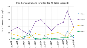
Figure 2: Iron concentrations for all sampling locations except Site B for January – December of 2023. Any “0” value for Site A represents below the detection limit of either 4 or 5 μg/L.
Some sites showed a seemingly opposite response in terms of iron concentration to the rain event, with Site A and Site D actually having an increase in their iron concentrations for the 4/28/23 samples. Site A also had a higher Fe concentration in the heavy rain month of July compared to June and August.
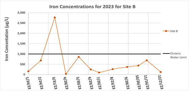
Figure 3: Iron concentrations for Site B only for January – December of 2023. The EPA chronic aquatic life limit of 1000 μg/L (13) is shown by the black line.
However, Site D did not show the same effect. It is worth noting that neither Site A nor Site D’s sampling locations had much visible red-brown microbial growth unlike Site B, which had extensive visible growth in March and lesser amounts of growth at other times of the year.
Manganese Results
The Mn concentrations for the water samples from Sites A, B’, C, and D for Jan. – Dec. 2023 are shown in Figure 4. Manganese concentrations at each site except Site B’ are higher and span a limited range in values during the dry months; wet months are characterized by lower manganese concentrations. Site B’ exhibited somewhat different behavior — manganese concentrations in January – April 2023 were lower (average 31.5 μg/L) whereas manganese concentrations later in the year (May – December) were higher (average 85.0μg/L).
Figure 5 is a separate graph for Site B because its high concentrations make it hard to see the distinct differences of the other sites all on one graph. Site B similarly had no particular trend of up or down, however it did have an outlier of particular note in March, which was at 1,234 μg/L, well above the average level for site B which is already much higher than the other sites. Note in Figure 3 that the Fe concentration at Site B on 3/31/2023 was very high as well. Manganese concentrations at Site B were also well above the recommended drinking water limit of 50 μg/L during the year, with the only exception being April, which was the rain event. The highest overall Mn concentration of 1,234 μg/L occurred on 3/31/23 in the sample from Site B.
The highest average concentration occurred at Site B with an average concentration and standard deviation of 344.4 ± 331.9 μg/L. The lowest average concentration occurred at Site C with an average concentration and standard deviation of 24.3 ± 13.3 μg/L.
When samples were collected on 4/28/23 there was a significant amount of rain, which heavily diluted the measured Mn concentrations at all sampling locations except Site C. July similarly had extensive rain throughout the month, however there was no rain on the day of collection. These results are generally reflected in the data, the only outlier being Site B’ in July, which was the highest concentration for Site B’.
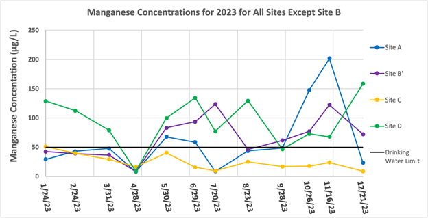
Figure 4: Manganese concentrations for all sampling locations except Site B for January – December of 2023. The EPA drinking water limit of 50 μg/L (12) is shown by the black line.
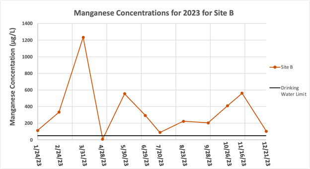
Figure 5: Manganese concentrations for Site B only for January – December of 2023. The EPA drinking water limit of 50 μg/L (12) is shown by the black line.
While data from all sampling locations for the year indicated a positive correlation between concentrations of iron and manganese (not shown, p<0.01, rho = 0.40), there was a particularly strong positive correlation between concentrations of iron and manganese for Sites B and B’ (p<0.001, rho =0.95) as shown in Figure 6.
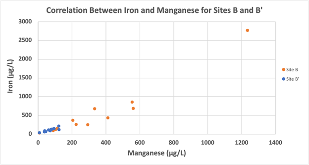
Figure 6: Iron and manganese concentrations for Sites B and B’ only for January – December of 2023 displayed a significant positive correlation (p<0.001, rho =0.95).
Chloride Results
As shown in Figure 7, there was no decreasing or increasing trend for chloride concentrations throughout the year. All sites are almost always above the chronic aquatic life limit for chloride except for Site C and at the other sites when there was above-average precipitation on the days leading up to, or on, the actual sampling date. Site C was above the limit only a few times throughout the year, including April, which was a rain event.
The highest average concentration occurred at Site D with an average concentration and standard deviation of 502.7 ± 206.8 mg/L. The lowest average concentration occurred at Site C with an average concentration and standard deviation of 177.3 ± 97.3 mg/L.
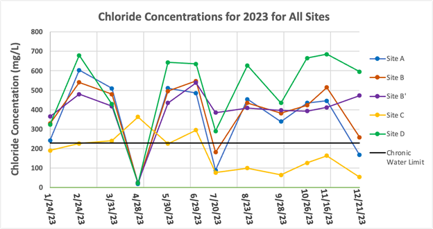
Figure 7: Chloride concentrations for all sampling locations for January – December of 2023. The EPA chronic aquatic life limit of 230 mg/L (13) is shown by the black line.
Chloride Comparisons with 2022
The chloride levels measured on the HCC campus in 2022 [26 and Pie and Carmody, unpublished data] were compared to the chloride levels from 2023 (this study). A comparison of the averages, standard deviations, low, and high chloride values at each site for 2022 and 2023 is shown in Table 3. The average and maximum chloride concentrations measured at each site were all higher in 2022 than in 2023. In fact, in 2022, there were five chloride measurements that exceeded the acute aquatic limit for chloride of 860 mg/L (all in the winter) whereas the highest chloride concentration measured in 2023 was 685 mg/L on 11/16/23 at Site D; while high, this is still well below the acute aquatic life limit.
In Figure 7, the chloride concentrations at each site define a more-or-less constant level throughout the year except during rainy periods when they dip downward from this level. These apparent levels have been quantified by taking the average chloride concentration for the eight “dry” months in 2023 (see Precipitation considerations section); these “dry month” averages are shown in Table 3.
| Chloride (2022, mg/L) | Chloride (2023, mg/L) | Chloride (Dry months in 2023, mg/L) | ||||
| lowest – highest | average +/- stdev | lowest – highest | average +/- stdev | lowest – highest | average +/- stdev | |
| Site A | 19.3 – 902.0 | 496.7+/- 267.1 | 17.7 – 603.4 | 358.3 +/- 186.8 | 242.2- 603.4 | 460.8+/- 103.2 |
| Site B | 21.3 – 1000.9 | 507.8 +/- 274.6 | 24.3 – 547.3 | 384.4 +/- 160.4 | 329.0 – 547.3 | 470.7+/- 72.7 |
| Site B’ | 28.0 – 564.5 | 424.5 +/- 180.7 | 25.7- 538.6 | 394.3 +/- 125.7 | 365.3 – 538.6 | 431.3+/- 54.5 |
| Site C | 72.8 – 951.3 | 275.6 +/- 309.6 | 53.8 – 363.1 | 177.3 +/- 97.3 | 99.6 – 295.5 | 196.2 +/- 64.2 |
| Site D | 84.4 – 1474.6 | 560.5 +/- 365.8 | 22.6 – 685.0 | 502.7 +/- 206.8 | 324.0 – 685.0 | 586.1 +/- 134.0 |
Table 3: Maximum, minimum, and average (with standard deviation) values for chloride in 2022, chloride (all) in 2023, and chloride in the eight dry months in 2023: January, February, March, May, June, August, October, and November. 2022 chloride data is from [26] and Pie and Carmody (unpublished data)
Correlations with Chloride
As shown in Figure 8, chloride and conductivity are strongly positively correlated with each other (p<0.001, rho =0.96) across all sites throughout the year. As chloride concentration increased, so did the conductivity.
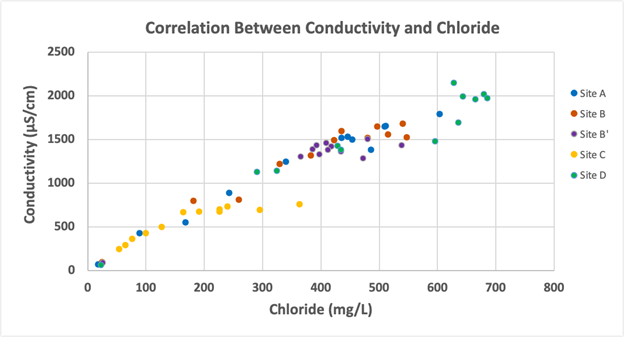
Figure 8: Conductivity levels and chloride concentrations for all sampling locations for January – December of 2023 displayed a significant positive correlation (p<0.001, rho =0.96).
For all sampling locations for the year, the concentration of manganese was positively correlated with the concentration of chloride (p<0.001, rho = 0.67) as shown in Figure 9.
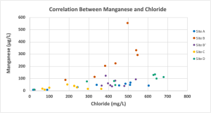
Figure 9: Manganese and chloride concentrations for all sampling locations for January – December of 2023 displayed a significant positive correlation (p<0.001, rho =0.67).
For sites B and B’ only, the concentration of iron was positively correlated with the concentration of chloride (not shown, p<0.01, rho = 0.58). However, no correlation between iron and chloride was observed when the data from all the sampling sites was combined for the year.
Nickel results
The nickel data for January – December 2023 are summarized in Table 2. All samples collected throughout the year had concentrations of Ni below the chronic aquatic life limit [12]. For Sites A and B’, nickel concentrations in all samples throughout the year were below the detection limit (<0.75 μg/L). Site B only had detectable Ni in May with a concentration of 0.98 μg/L. Site C had four months with Ni concentrations of above the detection limit with a range of 0.76 – 1.23 μg/L.
| Nickel Concentration (μg/L) | |||
| Sampling Locations | Lowest | Highest | Average +/- Stdev * |
| Site A | <0.75 μg/L | N/A | N/A |
| Site B | <0.75 μg/L | 0.98 | N/A |
| Site B’ | <0.75 μg/L | N/A | N/A |
| Site C | <0.75 μg/L | 1.23 | 1.01 +/- 0.18 |
| Site D | <0.75 μg/L | 10.12 | 5.49 +/- 2.23 |
Table 2: The highest and lowest Ni values recorded for each site as well as the average standard deviation. N/A means that no Ni was ever above the detection limit for that site.
*Average and standard deviations are calculated for concentrations above the detection limit.
Site D was the only sampling location with consistently measurable concentrations of Ni. The Ni concentrations for each month are shown on Figure 10. The only month that had below detection limit values of Ni for Site D was April, which was a rain event day. The highest concentration of 10.12 μg/L was measured in February with the colder months (December – March) having slightly higher concentrations than those in the warmer months.
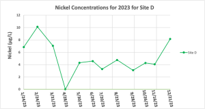
Figure 10: Nickel concentrations for all sampling locations for January – December of 2023 for just site D. The concentration of Ni in the water sample collected on 4/28/23 was below the detection limit of 0.75 μg/L.
Discussion/Conclusion
To further understand the quality of the water and metal concentrations within the stream systems on Howard Community College’s campus, this study examined the concentrations of three heavy metals (Mn, Fe, and Ni), Cl- concentrations, and other water quality parameters in five sampling locations within two different stream systems on campus monthly throughout 2023. The goals of the study were to build upon data collected from previous studies conducted on campus to compare values between years, to compare measured levels to water quality limits, examine the impact of the continued construction on campus, and examine correlations between parameters measured.
The 2021 and 2022 cycles of this research project found that Cl- concentrations were substantially higher in the winter months than they were during the rest of the year [25, 26]. However in 2023, that trend was not seen in the data, which is most likely due to the fact that there was almost no snow in the Baltimore-Washington area during the winter of 2022-2023, hence there was extremely limited application of salt and brine to the roads as well. However, despite this, concentrations of Cl- for 2023 are consistently above the chronic aquatic life limit for Cl-, with the exception of rainy months, which provides further support for the idea that removal of excess salt from groundwater may be a long-term process [15]. During dry months, the chloride concentrations at each site define a more-or-less constant level throughout the year. Considering the context of each site gives us a different meaning to this data. Site D is on a different stream system than Sites A and B (Figure 1) and Site D is highly disturbed by the proximity of impervious surfaces (parking lots and a parking garage) and a large construction site. The proximity to impervious surfaces and the runoff from them might explain why Site D typically has higher chloride concentrations than other locations. Site C is a pond and Site B’ is a culvert. However, the average dry-month chloride level at Sites A and B (461-471 +/- approx. 100 mg/L) may give an indication of the chloride concentration in the baseflow of this stream, that is, the chloride concentration in the groundwater in the northeast part of the HCC campus. If this is true, then the chloride level in the groundwater that feeds into the stream at Sites A and B is well above the chronic aquatic life limit and these concentrations are most likely having a detrimental effect on the ecosystem in and around this stream.
Iron concentrations at all sites were well below the chronic aquatic life limit, with the only exception being in March 2023 when a particularly high iron concentration was measured at Site B. This means that the streams on the HCC campus likely had Fe concentrations that are considered safe for aquatic life for most of the year. However, Mn concentrations at many sites over the year were above the EPA drinking water limit. Site C was the exception to this as it was consistently below the drinking water limit for Mn except for in January when the Mn concentration at Site C was 51.2 μg/L. This is more than likely due to the fact that Site C is a pond whereas all of the other sites are streams or culvert outflows. Mn levels are more diluted in the pond since a much greater volume of water is present. The other sites were usually above the drinking water limit for Mn with the major exceptions being the months of January through March for Sites A and B’, and rainy months, which significantly decreased the concentrations of Mn at most sites. This means, in terms of the average Mn concentration, that the stream water does not meet the secondary drinking water limits for most months of the year. The site with the highest Mn concentrations was Site B, which was well above the limit every month except for April, when it rained heavily on the day of sampling. There was also a significant spike in concentration at Site B in March, however it is not known what exactly caused this spike in concentration for that month. It is known that, at Site B and B’, the concentrations of Fe and Mn have a strong positive correlation with each other, which suggests that the concentrations of these two metals are being influenced by the same process at those sites. This may also relate to the fact that in the month of March, as well as other months, an orange/brown microbial growth was visible at Site B. This growth was not visible at other times of the year like on 7/20/23 when both Mn and Fe concentrations were low, but was appreciably extensive in March.
Although in most cases the measured concentrations of metals decreased during the wet months (July and December 2023) and during rain events (April 2023), in some cases, the opposite effect was observed. For example, the iron concentrations of samples collected at Site A on 4/30/2023 and 7/20/2023 were higher than expected. Radinsky and McMillian [25] made a similar observation for samples collected during a rain event on 8/17/2021. In this instance, Mn concentrations were lower in the 8/17/2021 samples whereas copper concentrations were higher in the samples from Sites A and B. These authors suggested that Mn originates primarily from groundwater whereas the high copper concentrations resulted from runoff from parking lots, with the copper originating (presumably) from the degradation of vehicles parked on those lots. A rain event dilutes the groundwater component (Mn) of the water in the stream but, on the other hand, washes other metals (Cu) into the streams that have accumulated on the surface of the parking lots. A similar explanation may apply for the higher iron concentrations measured at Site A, which is the closest sampling site to parking lot A on the HCC campus, on 4/30/2023 and 7/20/2023.
Measurable amounts of Ni (3.1 to 10.1 μg/L) also occurred consistently only at Site D which is the closest to the active construction site. Ni at the other sampling sites was mostly below the detection limit. This, along with the heightened turbidity at Site D suggests that the nearby construction site is having a direct, negative effect on the stream system. Ni was also measured at these sites in 2022 [26]; this study found detectable Ni concentrations at Site B from January – May 2022 and detectable levels of Ni at Site C from January – July 2022, during the same time of year when chloride and conductivity were higher. This suggests that Ni is another metal that is being released from adsorption sites in response to higher chloride concentrations. A larger sample size of water samples with detectable Ni would be needed in the future to better examine if there is a statistical correlation between Ni and Cl-. Ni may not be above the EPA chronic or acute aquatic life limits, but the turbidity at Site D did get to a level which is considered unacceptable by MD state standards, in that it reached 163.8 one month and state policy dictates that it cannot go over 150 at any point in time as a direct result of discharge [27].
The results of this study suggest that chloride concentrations in the streams on the HCC campus are above the chronic aquatic life limit (230 mg/L) for most of the year and that degradation of the ecosystems of these streams should be expected as a result. Furthermore, as noted and observed by other researchers [2], elevated levels of chloride in soil- and groundwater have been linked with elevated levels of metals as well. In this study, we have documented levels of Mn above the drinking water limit for most of 2023 (particularly May 2023 onward) and levels of Fe which, while generally are below the chronic aquatic life limit of 1000 μg Fe/L, might eventually be cause for concern. Future work will focus on the microbes and the carbonate rocks present at Site B to try to elucidate how either or both of these are contributing to the particularly high Mn and Fe levels observed at this site.
Supplementary Data
A more comprehensive data set can be found at: https://docs.google.com/spreadsheets/d/10GUuQHRAAHHHrbl8P5zYcFvVCFYgp2X11Loqk0QeTrs/edit?usp=sharing
Acknowledgements
I would like to thank first and foremost my mentors Dr. Carmody and Dr. Pie, without whom this project and paper never would have happened. I also wish to thank Belle Larson for her participation in this project during the Spring 2023 semester. I would also like to thank HCC’s Department of Science, Engineering, and Technology and everyone involved in the undergraduate research program which gave me the opportunity to do this in the first place.
Contacts: stephen.shaner@howardcc.edu; hpie@howardcc.edu; rcarmody@howardcc.edu
References
[1] A. Müller, H. Österlund, J. Marsalek, and M. Viklander, “The pollution conveyed by urban runoff: a review of sources,” Science of The Total Environment, vol. 709, p. 136125, Mar. 2020, doi: https://doi.org/10.1016/j.scitotenv.2019.136125.
[2] M. S. Schuler and R. A. Relyea, “A review of the combined threats of road salts and heavy metals to freshwater systems,” BioScience, vol. 68, no. 5, pp. 327–335, Mar. 2018, doi: https://doi.org/10.1093/biosci/biy018.
[3] W. D. Hintz, L. Fay, and R. A. Relyea, “Road salts, human safety, and the rising salinity of our fresh waters,” Frontiers in Ecology and the Environment, vol. 20, no. 1, pp. 22-30, Feb. 2022, doi: https://doi.org/10.1002/fee.2433.
[4] S. Löfgren, “The chemical effects of deicing salt on soil and stream water of five catchments in southeast Sweden.,” Water Air and Soil Pollution, vol. 130, no. 1/4, pp. 863–868, Aug. 2001, doi: https://doi.org/10.1023/a:1013895215558.
[5] W. D. Hintz and R. A. Relyea, “A review of the species, community, and ecosystem impacts of road salt salinisation in fresh waters,” Freshwater Biology, vol. 64, no. 6, pp. 1081–1097, Mar. 2019, doi: https://doi.org/10.1111/fwb.13286.
[6] S. S. Kaushal, “Increased salinization decreases safe drinking water,” Environmental Science & Technology, vol. 50, no. 6, pp. 2765–2766, Feb. 2016, doi: https://doi.org/10.1021/acs.est.6b00679.
[7] S. L. O’Neal and W. Zheng, “Manganese toxicity upon overexposure: a decade in review,” Current Environmental Health Reports, vol. 2, no. 3, pp. 315–328, Jul. 2015, doi: https://doi.org/10.1007/s40572-015-0056-x.
[8] P. Cadmus, S. F. Brinkman, and M. K. May, “Chronic toxicity of ferric iron for north american aquatic organisms: derivation of a chronic water quality criterion using single species and mesocosm Data,” Archives of Environmental Contamination and Toxicology, vol. 74, no. 4, pp. 605–615, 2018, doi: https://doi.org/10.1007/s00244-018-0505-2.
[9] Z. Wang et al., “Acute and chronic toxicity of nickel on freshwater and marine tropical aquatic organisms,” Ecotoxicology and Environmental Safety, vol. 206, p. 111373, Dec. 2020, doi: https://doi.org/10.1016/j.ecoenv.2020.111373.
[10] C. Camaschella, “Iron deficiency,” Blood, vol. 133, no. 1, pp. 30–39, Jan. 2019, doi: https://doi.org/10.1182/blood-2018-05-815944.
[11] G. Cairo, F. Bernuzzi, and S. Recalcati, “A precious metal: iron, an essential nutrient for all cells,” Genes & Nutrition, vol. 1, no. 1, pp. 25–39, Mar. 2006, doi: https://doi.org/10.1007/bf02829934.
[12] US EPA, “National recommended water quality criteria – aquatic life criteria table,” www.epa.gov, Sep. 03, 2015. http://www.epa.gov/wqc/national-recommended-water-quality-criteria-aquatic-life-criteria-table (accessed Feb. 21, 2024).
[13] US EPA, “Secondary drinking water standards: guidance for nuisance chemicals,” www.epa.gov, Sep. 02, 2015. http://www.epa.gov/sdwa/secondary-drinking-water-standards-guidance-nuisance-chemicals (accessed Feb. 21, 2024).
[14] M. Cempel and G. Nikel, “Nickel: a review of its sources and environmental toxicology,” Polish Journal of Environmental Studies, vol. 15, no. 3, pp. 375–382, Jan. 2006.
[15] S. S. Kaushal et al., “Freshwater salinization syndrome: from emerging global problem to managing risks,” Biogeochemistry, vol. 154, no. 2, pp. 255–292, Apr. 2021, doi: https://doi.org/10.1007/s10533-021-00784-w.
[16] H. A. Dugan et al., “Salting our freshwater lakes,” Proceedings of the National Academy of Sciences, vol. 114, no. 17, pp. 4453–4458, Apr. 2017, doi: https://doi.org/10.1073/pnas.1620211114.
[17] R. B. Baird, A. D. Eaton, and E. W. Rice, Eds., Standard methods for the examination of water and wastewater, 23rd ed. Washington: APHA , 2017.
[18] J. Milivojević, D. Krstić, B. Šmit, and V. Djekić, “Assessment of heavy metal contamination and calculation of its pollution index for Uglješnica River, Serbia,” Bulletin of Environmental Contamination and Toxicology, vol. 97, pp. 737-742, September 2016, DOI 10.1007/s00128-016-1918-0. (Accessed Feb. 23, 2024).
[19] M. Varl and B. Şen, “Assessment of nutrient and heavy metal contamination in surface water and sediments of the upper Tigris River, Turkey,” Catena, vol. 92, pp. 1-10, May 2012, DOI: 10.1016/j.catena.2011.11.011. (Accessed Feb. 23, 2024).
[20] B. Sharma and S. Tyagi, “Simplification of metal ion analysis in fresh water samples by atomic absorption spectroscopy for laboratory students,” Journal of Laboratory Chemical Education, vol. 1, no. 3, pp. 54–58, 2013. (AccessedFeb. 23, 2024).
[21] Shimadzu Corp. (Analytical Applications Dept.), Atomic absorption cook book no. 4: electro-thermal atomic absorption spectrometer’s parameter for each element (AA-7000). Tokyo: Shimadzu Corp., 2010.
[22] D. C. Harris, Quantitative chemical analysis, 7th edition. US: W. H. Freeman, 2006.
[23] “5.7 nitrates,” EPA, https://archive.epa.gov/water/archive/web/html/vms57.html (accessed Apr. 26, 2024).
[24] D. Litke, “Review of phosphorus control measures in the United States and their effects on water quality,” U.S. Geological Survey, 1999. doi:10.3133/wri994007
[25] S. Radinsky and P. McMillian “A Year in the life of two campus streams: impact from road salt, ground water, and surface water contributions,” Journal of Research in Progress, vol. 5, pp. 35-56, May 2022. https://pressbooks.howardcc.edu/jrip5/chapter/a-year-in-the-life-of-two-campus-streams-impact-from-road-salt-ground-water-and-surface-water-contributions/
[26] H. Pie, R. W. Carmody, and A. M. Caraballo, “A tale of two streams: chloride, conductivity, and trace metals in streams on the HCC campus” GSA Joint Northeastern & Southeastern Section Meeting Reston, VA, 2023: https://gsa.confex.com/gsa/2023SE/meetingapp.cgi/Paper/385921.
[27] “SEDIMENT-related criteria for surface water quality.” Available: https://19january2017snapshot.epa.gov/sites/production/files/2015-10/documents/sediment-appendix3.pdf