Download a pdf of this paper

Abstract

Freshwater rivers and streams are as essential to our environment as blood vessels are to the human body, and because of its fluid nature, water chemistry and quality can be influenced by naturally occurring and anthropogenic events. From February 2021 to January 2022, our research team assessed freshwater chemistry at five locations on the campus of Howard Community College (HCC). We observed trends in water quality parameters, including chloride (Cl), pH, turbidity, temperature, conductivity, and dissolved oxygen levels as well as concentrations of manganese (Mn) and copper (Cu) ions. We found a positive correlation between manganese and conductivity levels when examining all samples collected throughout the year. The concentration of manganese appears to be highest during the winter months; the highest observed reading occurred in December 2021, and was nine times above the Environmental Protection Agency (EPA) drinking water recommendation of 50 µg/L [1]. The concentration decreases through spring. The lowest levels we observed were in summer, which for some sites were below the EPA recommendation. Correspondingly, chloride concentrations were highest during the winter months. These trends suggest the streams on campus may be impacted by the use of de-icing salts containing chloride in winter, according to a study that examined the effects of salt on the mobilization of metals like manganese [2]. Concentrations of copper generally remained consistent and below 2 µg/L, which is considerably lower than the EPA limit of 1.3 mg/L in drinking water [3]. Our data will serve as a baseline and allow us to observe changes in water quality and levels of trace metals that may occur as a result of road salt use and planned campus construction.

Introduction

Two streams begin near the campus of Howard Community College [4]. These streams are fed by local groundwater and stormwater runoff from on-campus and nearby surfaces, and supply the Little Patuxent River [5]. Columbia, Maryland is a densely populated suburb located between Baltimore and Washington DC, and within the watershed of the Patuxent River. Much of the Patuxent River basin is significantly urbanized, with population centers like Columbia experiencing rapid development over the last several decades. Developer James W. Rouse promised that the planned community would “fit naturally into the Howard County landscape, preserving the stream valleys, protecting the hills and forests, and providing parks and greenbelts” [6]. The Rouse vision capitalized on the natural beauty, weaving community into the landscape. Although streams and ponds, such as those on HCC’s campus, are aesthetic, recreational, and sociocultural assets to communities [7], research has shown that human activity in and around streams decreases the quality of freshwater and can threaten the health of the aquatic and terrestrial ecosystems they sustain [8].

The ecological value of freshwater is contingent upon its quality, and several global studies have found that anthropogenic activity decreases the quality of surface water [9] and groundwater [10-12]. Anthropogenic events such as rapid urbanization and development [9], industrial activities [11], the application of fertilizers [13], and stormwater runoff from impervious surfaces can alter the chemistry of nearby streams and rivers. Chemical changes can include contamination of heavy metal ions [10-12], an increase in chloride ion concentration, and conductivity [13-14]. Changes such as these can be caused by a combination of anthropogenic and geogenic occurrences [2, 15-16].

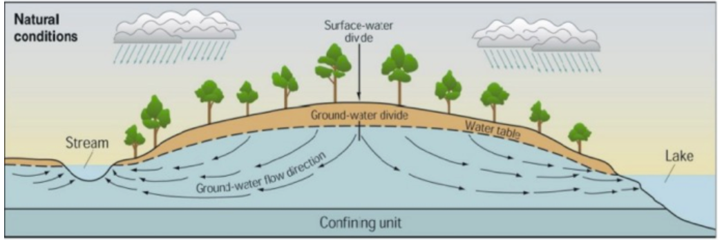
Freezing precipitation typically occurs from December to March in Maryland [17], and road salts are used ubiquitously. Research suggests that the application of road salts and de-icing substances are environmentally damaging anthropogenic activities because of their potential to increase the conductivity of freshwater and cause the mobilization of naturally-occurring metal ions in soil [2, 15]. After de-icing salt is applied to roads, melting ice and snow wash the salt onto the earth adjacent to the road surface. The water, now with a high salt concentration, is absorbed into the earth where it becomes dispersed through soil and, in time, percolates into the groundwater [10]. The sodium (Na+) and chloride (Cl-) ions from the dissolved salts promote the dissolution of metals, such as manganese [15], from soil or bedrock [18]. The metal ions can then become dissolved into the groundwater [2], which supplies freshwater streams [10] (Figure 1), such as those that begin around HCC’s campus. The salts can also lead to an increase in conductivity of freshwater [15-16]. Elevated concentrations of heavy metals and chloride ions can alter ecosystems and reduce biodiversity as species that are unable to adapt do not thrive and reproduce [5, 16]. Periodic testing of at-risk freshwater is recommended to maintain the integrity of the ecosystem it sustains and protect other river networks it supplies.

The Maryland Stream Waders, a volunteer group under the direction of the Maryland Department of Natural Resources, conducts monitoring of the freshwater rivers and streams in the area. The group evaluated the water quality of one of the streams on HCC’s campus in March 2019, and found elevated conductivity and nitrite concentration, and rated the campus streams with a score of 2 (out of 5) indicative of “poor” water quality after assessing collected water samples [20]. The streams on HCC’s campus flow into the Little Patuxent River. The Little Patuxent River is one of the major tributaries of the Patuxent River basin, an ecologically and economically crucial watershed in Maryland [21]. The basin supplies the Triadelphia and Rocky Gorge reservoirs [21-22], which according to the Washington Suburban Sanitary Commission (WSSC) supplies drinking water to 650,000 Maryland residents [23]. The Patuxent River empties into the Chesapeake Bay, the largest estuary in the United States, and NOAA fisheries estimates that the Bay produces about 500 million pounds of seafood each year [24]. In 2019, the Patuxent Rivers Watershed Group stated in their annual report that between 1990 and 2019 levels of chloride and sodium ions have increased two to three times in the Rocky Gorge Reservoir, and the group issued a recommendation to limit and manage the use of road salts in the Patuxent River Watershed, “before water quality standards are exceeded” [21].

Copper is a soft, naturally-occurring metal that is used in electrical wiring, plumbing, and industrial settings [25], and aids in biological function [26]. As a trace metal, it is essential for human health and homeostasis, yet has a cumulative effect in mammalian organs and tissues if consumed in excess. On the biochemical level, copper toxicity can cause free radical-induced oxidative damage to cells; affected organisms experience gastrointestinal and neurological disorder [26]. Without chelation therapy to remove copper from the body, an accumulation of copper can lead to renal and cardiac failure, hepatic necrosis, and death [26]. The EPA has identified that most copper found in drinking water originates from copper plumbing, and has classified copper as a regulated drinking water contaminant [3] because of its toxicity, and as a nuisance chemical because of its metallic taste and blue-green staining [1]. The EPA permits a maximum of 1.3 mg/L in drinking water [3].

Manganese is also considered a biologically essential nutrient, and is vital for hormone signaling and the function of connective tissues such as cartilage and bone. Unlike copper, manganese has a low potential for acute toxicity and is considered noncarcinogenic, but it has biological potential to cause homeostatic disturbance [27]. If consumed or inhaled over extended periods of time, such as in the case of occupational exposure or drinking from contaminated well water [28-29], elevated concentrations of manganese in the body can cause nervous system disorders such as manganism and parkinsonism, which are characterized by movement abnormalities, deterioration of motor skills, and speech difficulties [27]. The occurrence of manganese toxicity is low [28], and the EPA has set the maximum allowable level of manganese in drinking water at 50 µg/L on the basis of aesthetics; it can cause unattractive staining on surfaces and fabrics [1]. At this time, the EPA does not have a recommendation for concentrations of manganese in freshwater [30] and research on the chronic effects of manganese toxicity on freshwater systems in the United States is limited.

Our investigation of heavy metals and conductivity levels of the soil and water of the streams and pond on HCC’s campus continues and expands the scope of research conducted by three other groups of staff and students of HCC. Between fall 2017 and 2020, the teams observed conductivity levels exceeding the ideal range for freshwater streams and concentrations of chloride that are above what is recommended for aquatic life [13-14], which corroborates the 2019 assessment by the Maryland Stream Waders. Additionally, Beckjord and Straube noted pollution-level concentrations of NO₃– between 2017 and 2018 [13], and Carmody and Mai found elevated concentrations of manganese in the spring of 2020 [31]. Each group recommended further monitoring of the streams and pond, and our research goals were designed under this direction. We hope that the cumulative results of all research groups can be used for future comparative studies regarding how the water quality and concentrations of heavy metals changes on campus as the campus itself evolves, such as the current construction of the new Mathematics and Athletics Center (MAC) building, which began in 2021.

Methods

Preparation of materials

Prior to use all sampling and filtration materials are washed with lab detergent and tap water, rinsed three times with deionized water, soaked in 4% nitric acid (HNO₃), rinsed three more times with deionized water, and oven dried at 50ºC. This thorough process was developed based on procedures utilized by similar studies in Turkey in 2016 [11] and India in 2013 [32], and is intended to remove dissolved metallic residues and other impurities that may interfere with the sensitive metal analysis of the samples. During transport to sample locations, sample bottles are kept in plastic bags to prevent contamination in the field.

Sample collection

Samples of freshwater were collected from four locations on the campus of HCC once a month from 2/25/2021 to 1/13/2022, between 10:00 am and 3:00 pm. Sampling at Site B′ began on 6/10/2021, and this location was added to gather more data about the input into Site B from the water flowing in from the adjacent culvert, which is a concrete tunnel that passes under Little Patuxent Parkway. The locations (Figure 2) were selected because of their accessibility and proximity to impervious surfaces and stormwater drainage culverts. Environmental conditions at each location were measured, including time of sampling, air temperature, air pressure, dissolved oxygen (DO) levels, and the maximum depth of the water. Air temperature was measured with a Vernier LabQuest temperature probe, air pressure was measured with a Vernier LabQuest Barometer, DO was measured with a Vernier LabQuest Optical DO Probe, and water depth was measured with a standard ruler. Between measurements the probes are rinsed with deionized water to minimize microbial contamination between sample locations. Environmental notes and observations were also recorded at each location.

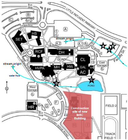
Site A and Site B are located in a small wooded area on campus between Scholarship Drive and Faculty Drive, south of Little Patuxent Parkway. A stream begins just west of this location, and runs parallel to the parkway, and continues off campus. Site A is located closest to the stream origin. Throughout most of the year, especially during extended periods of low precipitation in the summer, the stream at Site A often had low water flow.

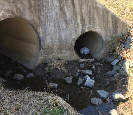
Site B is situated about 18 meters downstream of Site A, and is characterized by higher water flow and stream depth than Site A. At Site B, a culvert empties into the stream (Figure 3a), and sample water was collected downstream from the culvert. Beginning in June 2021, water samples were also collected from the water flowing from the culvert to allow us to characterize both sources of water that combine at Site B and about how water from this culvert may affect water quality and metal ion concentrations in the stream at Site B. This location was named Site B′.

Another stream crosses through HCC’s campus, beginning off-campus near a medical office complex and continuing south of the quad. The stream crosses under Campus Drive via metal culverts, and runs through a low-lying area before emptying into the campus pond. Site C is located on the north shore of the pond, a location with significant wildlife activity. Throughout the year, Canada geese were seen around the pond, and frogs and small fish were observed in the pond in the summertime months. Felled and damaged trees on the shore of the pond and a visible dam were evidence of a local beaver population.

Site D is located at a culvert (Figure 3b) that allows the stream to pass under Campus Drive before the stream feeds into the pond. At this location water flows year-round, with increased water volume noticed following heavy precipitation events. Despite its proximity to campus buildings, a high-volume road, and frequent evidence of human trash, wildlife was seen numerous times throughout the year, and included ducks, geese, frogs, and crayfish.

Two samples were collected at each primary location: one in a 1 L polyethylene bottle and another in a 250 mL polyethylene bottle for additional water quality analysis. Samples from Site B′ were collected with two 250 mL bottles. To collect a sample, nitrile gloves were worn, and the bottle was submerged to a depth of 10 cm where the lid was removed, and the lid was replaced while underwater to prevent contamination from the air or surface of the water. At Site C, to accommodate deeper water, rubber dishwashing gloves are worn during sample collection and water quality measurements. After collection, the bottles were stored on ice until returned to the lab.

Sample filtration, acidification, and storage

Sample water collected in 1 L polyethylene bottles was used for testing the presence of heavy metal ions. Polyethylene was selected to avoid contamination of samples via metal leaching from the container [32]. Samples were filtered via vacuum filtration to remove organic particulates and sediment, allowing us to examine dissolved metals. A MF-millipore filter with 0.45μm pore size was used. Before sample water was filtered, 100 mL 2% HNO₃ was run through the apparatus and filter paper to remove any metal ions that may have contaminated the equipment after washing and drying. This volume is then transferred to a clean 250mL polyethylene bottle, labeled as a filter blank with the date and location of the sample that was to be filtered in the apparatus. The filter blank was later tested for metal contamination from the lab. Sample water from one location was then filtered through the filtration apparatus, and if necessary, the filter was changed as many times as needed to fully filter each 1 L sample. The first filter from each location was saved, labeled, and refrigerated in polystyrene petri dishes for analysis in follow up research. For this project, the filters were not analyzed and only used for filtration.

Each filtered sample from Sites A, B, C, and D was then transferred to a new, clean 1 L polyethylene bottle and acidified with 2 mL 70% HNO₃, and samples collected from Site B′ were acidified with 0.5 mL 70% HNO₃ to bring the pH in the filtered samples to below 1. Acidifying the samples eliminates any remaining microbes that passed through filtration, as microbe metabolism can alter the chemistry of the samples, and helps keep metal ions suspended in water and not accumulate into precipitate. The samples were then labeled and refrigerated until ion analysis.

Water quality analysis

Water collected from each location in 250 mL polyethylene bottles were used to assess the original water quality of each location, and therefore were not filtered or acidified. For each sample, several parameters were measured, including pH, turbidity, conductivity, and chloride ion concentration, using pre-calibrated sensors and probes. The pH was quantified using a Vernier LabQuest pH Sensor, turbidity was measured using a Vernier LabQuest Turbidity Sensor, conductivity was measured using a Vernier LabQuest Conductivity Probe, and chloride ion concentration was measured using a Vernier LabQuest Chloride Ion-Selective Electrode Probe. A new chloride sensor was introduced on 1/13/22, and new conductivity standards were used for a more complete calibration curve.

Metal ion analysis with AAS

Atomic absorption spectroscopy (AAS) was used to determine the presence and concentration of metal ions in samples [33]. These analyses were conducted using a Shimadzu AA-7000 spectrophotometer equipped with a graphite furnace with either a high density graphite tube or a pyrolytic graphite tube as well as manganese and copper hollow-cathode lamps. For manganese analysis, a wavelength of 279.5 nm was used [34]; for copper, the wavelength was set to 324.8 nm [35]. In order to increase the sensitivity for measuring copper in the water samples, the graphite tube used was switched to a pyrolytic graphite tube in August 2021. Data was sent directly from the spectrophotometer to an adjoining computer, where calculations were completed and graphs were generated via Shimadzu WizAArd software [34]. The software was also used to set parameters for analyzing different metals.

Samples were pipetted into labeled cuvettes, which were then seated in the rotating cassette of the spectrophotometer autosampler. A micropipette tip was inserted into each individual sample, and a small volume was transferred via capillary inlet tube into the spectrophotometer. The autosampler micropipette was automatically rinsed by the instrument between samples to prevent cross-contamination. The sample was heated via graphite tube and the metal ions were atomized and irradiated with light from the hollow-cathode lamp specific for that elemental analysis. The amount of light that was absorbed by the atomized metals in the sample is detected and sent to the computer [33]. AAS was used to determine the concentration of specific metals in solution by measuring the absorbance of a particular wavelength of light by each sample. According to Beer’s Law (Equation 1), the absorbance of light is directly proportional to concentration in solution, and therefore a formula can be used to determine concentration from absorbance [33].

[latex]A=\varepsilon{bC}[/latex]     (1)

where A is absorbance, ɛ is molar absorptivity, b is length of light path, and C is concentration.

The sample was analyzed three or four times depending on the reproducibility of the first three measurements, and the absorbance was averaged and recorded by the WizAArd software. When analyzing manganese, after each water sample a sample of trace metal grade 2% HNO₃ was run through the system three to four times to remove any residual metal ions from analysis of the previous sample. This was not needed when analyzing copper concentrations in water samples as those concentrations were low enough not to carry over between samples. When testing for manganese, samples had to be diluted by a factor of 2 to 50 depending on the starting concentration to bring the absorbance into the linear, calibrated range of the AAS. A trace metal grade solution of 2% HNO₃ was used to dilute samples, as HNO₃ is recommended for keeping metal ions suspended in solution. The concentration values obtained from the absorption of diluted samples was then multiplied by the appropriate dilution factor to determine the undiluted concentration of metal in the original sample.

Calibration curve

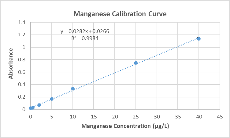
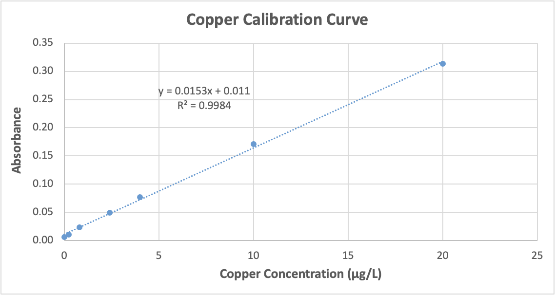
A calibration curve (Figure 4) is a display of data from analysis of known quantities of analyte [33], and this linear approach was used to determine the unknown concentration of metal ions in freshwater samples. Calibration curves for manganese (Figure 4) and copper (Figure 5) were created based on the analysis of a series of standard solutions created from 1000 mg/L stock solutions from Inorganic Ventures. Manganese standard solutions containing 0.5, 2, 5, 10, 25, and 40 μg/L were used; copper standard solutions had 0, 0.24, 0.80, 2.4, 4.0, 10, and 20 μg/L. Spectrophotometer data for each series of solutions showed a linear response [33], allowing us to determine the absorption of unknown samples with linear regression.

On August 16, 2021 the high density graphite tube in the AAS was switched to a pyrolytic graphite tube to obtain better sensitivity when analyzing copper. This resulted in a shift in measurable manganese concentrations and new standards containing 0.5, 1.0, 2.5, 5.0, 10.0, and 15.0 μg/L were created and used. All water samples were appropriately diluted to account for this new range.

Results

Manganese levels & trends

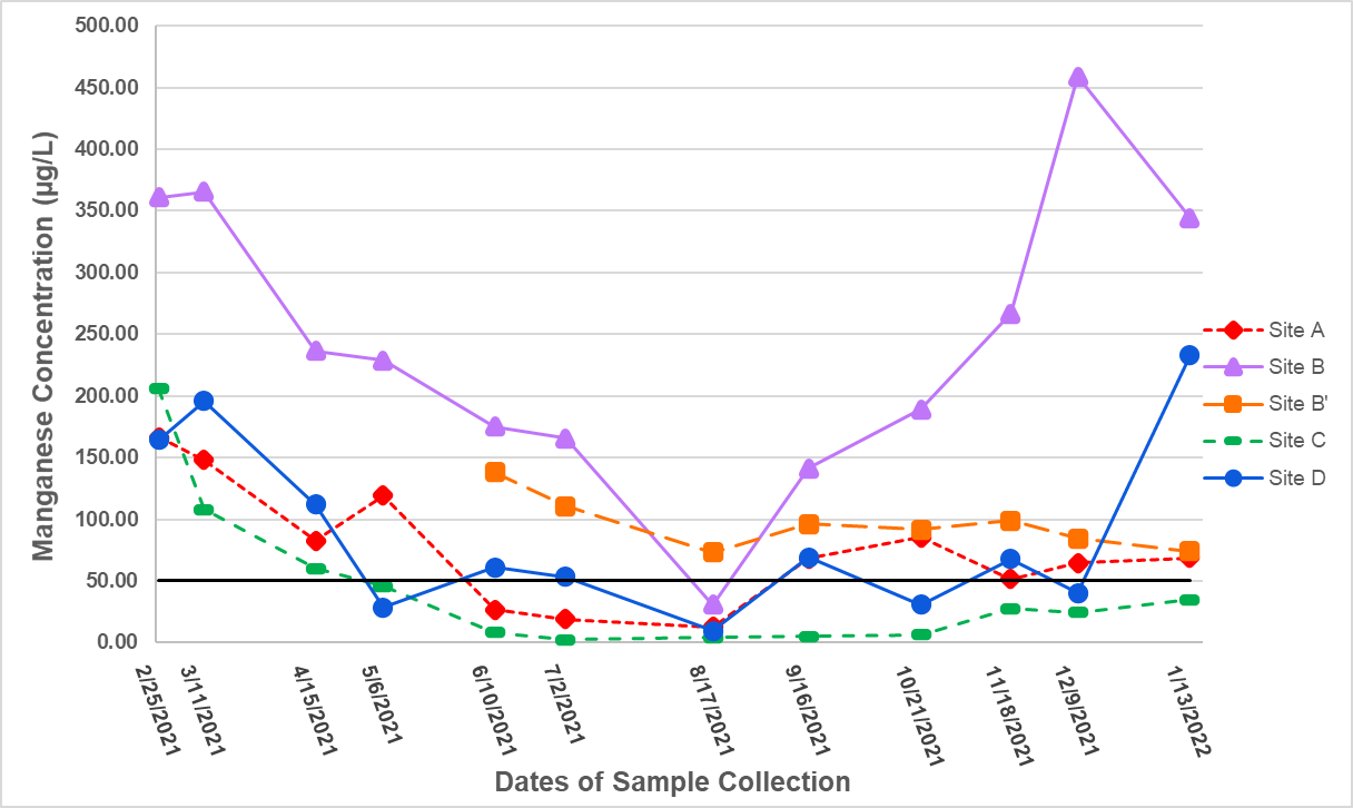
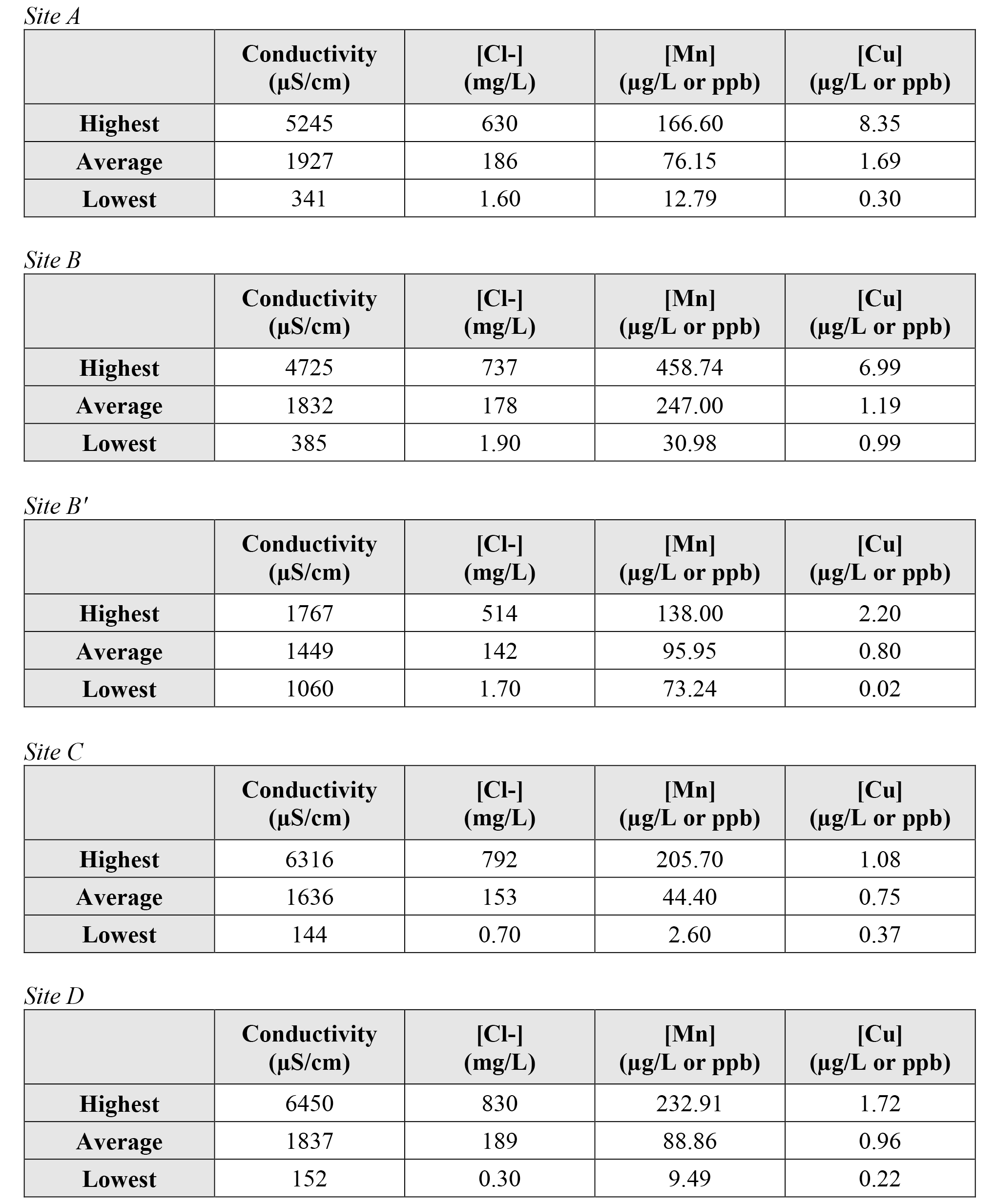
Ranges of manganese concentrations varied between the different sites from February 2021 to January 2022. Sites A, B, C, and D all displayed a trend of decreasing concentration from winter into summer, however, only sites B and C displayed an increase again in late fall of 2021 and early winter 2022. Site C, the pond, appeared to have the lowest concentration of manganese overall with an average and standard error of 44.40 ± 17.30 µg/L, and was the site of the lowest observed concentration during the observation period (2.60 µg/L on 7/2/2021). Manganese was consistently highest at Site B, and the highest observed reading overall was at this location, recorded at 458.74 µg/L on 12/9/2021. This location had an average year-round manganese concentration and standard error of 247.00 ± 34.29 µg/L. The lowest manganese concentration for Site B occurred on 8/17/2021 where sampling occurred after a precipitation event.

Copper levels & trends

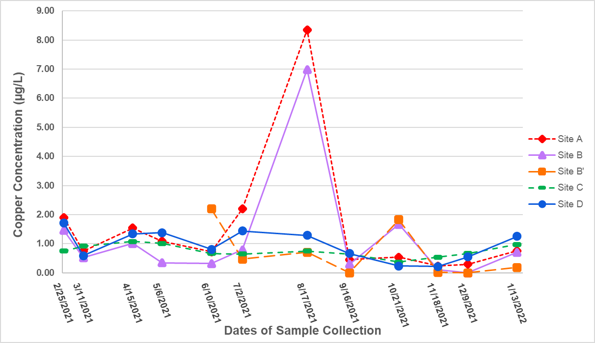
Concentration of copper at all locations from February 2021 to January 2022 remained far below the EPA limit of 1.3 mg/L for drinking water [3]. The highest concentration observed was 8.35 µg/L at Site A on 8/17/2021 (Figure 7), and the second-highest concentration overall also occurred that day at Site B (6.99 µg/L). It should be noted that samples were collected during a precipitation event on this day. For the most part, on days without precipitation, concentrations of copper at our sampling sites remained below 2.00 µg/L throughout the year. Excluding data from Sites A and B on 8/17/2021, the average and standard error for all samples was 0.86 ± 0.08 µg/L. The lowest detectable concentration was 0.02 µg/L at Site B′ on 11/18/2021. However, there were three samples that contained concentrations of copper below the detection limit: Site B’ on 9/16/21, Site B′ on 12/9/21, and Site B on 12/9/21.

Chloride levels & trends

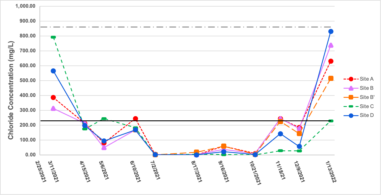
Chloride concentration demonstrated a trend similar to that of manganese, as seen in Figure 8. Concentrations of chloride at all sites examined in March 2021 were above the recommended chronic exposure limit of 230 mg/mL [36] with the highest measurement being 791 mg/L at Site C. A general trend of decreasing chloride concentration from March 2021 through late summer was observed, and lowest concentration recorded was 0.70 mg/L on 6/2/2021 at Site C. It should be noted that testing for chloride began in March 2021, although sampling and data collection began in February of that year. Chloride levels increased again the following late fall and winter. In January 2022, the highest recorded concentration was 830 mg/L (Site D), and all sites that day had chloride levels that were above the chronic exposure limit of 230 mg/L [38], except for Site C at 229 mg/L. Overall, all samples measured for the year were below the acute exposure limit for chloride of 860 mg/L [36].

Conductivity levels & trends

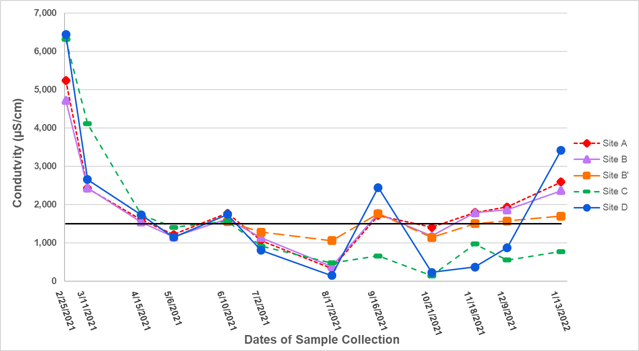
Conductivity varied annually with a trend similar to that of manganese and chloride, with variations throughout the observation period. Overall the highest levels were observed in winter months, and the highest reading of all locations was 6450 µS/cm at Site D on 2/25/2021. Despite increases in levels on 6/10/2021 and again on 9/16/2021, the lowest readings generally occurred in summer and fall; the overall lowest reading observed was 144 µS/cm on 10/21/2021 at Site C. Conductivity averaged 1623 µS/cm from February 2021 to January 2022, which is above the upper range of what is considered typical and healthy for freshwater. The EPA notes that conductivity of rivers and streams in the United States typically ranges from 50 to 1500 µS/cm [37], and conductivity under 300 µS/cm is considered ideal for a healthy freshwater environment in the central Appalachian region [38].

Other measures of water quality

Water quality parameters were measured at each location, and include pH, water temperature, dissolved oxygen levels, and turbidity. We have chosen to provide pH and other measures of water quality not shown here within supplementary data present at the end of this paper. This data was collected to provide more information on the complete health profile of the streams and pond and for comparative analysis in future research. In this investigation, these parameters were not used in correlation analysis.

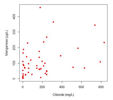
Correlation between manganese concentration and conductivity

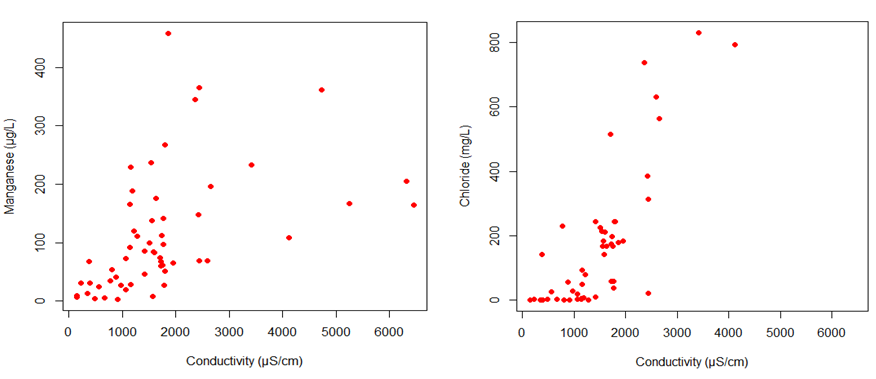
A comparison of manganese concentrations and conductivity were plotted via scatter plot (Figure 10). A Spearman’s correlation test was conducted using the R statistical software. This revealed a significant positive correlation between the conductivity and manganese concentrations (rho=0.653, p-value <0.001). This plot shows that as conductivity increases, manganese concentration also increases, which suggests that the primary ions that drive conductivity levels could be causing manganese concentrations to increase in the stream systems on campus. Furthermore as shown in Figure 10, chlorine concentrations were positively correlated to conductivity levels (rho=0.652, p <0.001), which suggests that chloride ions are a primary driver of conductivity. Figure 11 shows that there is a weak positive correlation between manganese and chloride; more data is needed to further define this relationship. It is also possible that this correlation is less strong than that between manganese and conductivity because there are other ions in addition to chloride that influence the concentration of manganese.

Discussion

Past studies conducted by faculty and students of HCC have monitored freshwater on campus and have explored the effects of anthropogenic activities on the water quality. Beckjord and Straube monitored the streams on campus from fall 2017 to spring 2019 and observed an average conductivity of 6256 µS/cm that winter. It was suggested a cause could be the use of de-icing salts [13]. The following year, Wortman and Erickson further explored the effects of anthropogenic activities, and specifically assessed the impact of legacy pollution on conductivity levels in the soil and freshwater on campus. They observed median conductivity levels of 1733 µS/cm and 1973 µS/cm in the freshwater on campus, and identified a correlation between conductivity levels and chloride concentration. They suggested de-icing salts as the primary source of elevated chloride contamination, and suggested that the higher concentrations of chloride correlate with higher conductivity concentrations [14]. Our analysis of conductivity and chloride concentrations revealed trends similar to those observed in campus freshwater from 2017 to 2020. It appears that conductivity and chloride ion concentrations are highest in the wintertime months, which suggests contamination of de-icing road salts from the many roads, walkways, and parking lots on and around the college campus. More data is necessary to clarify this correlation.

In March, August, and October 2020, Carmody and Mai assessed surface water quality and also began documenting the presence of heavy metals in the streams on campus. Manganese and copper ions were identified and preliminary trends in concentrations of these metals were discovered. The concentrations measured during their observation period are similar to what we observed: higher concentrations that were above the EPA recommendation in late winter and lower concentrations in late summer and fall. During our monitoring, we noted manganese concentrations were above EPA recommendations for much of the year at all sites except Site C, which was only observed above the recommendation in February to April 2021. Site C could perhaps have lowered concentrations due to being a pond and the largest body of water on campus. Manganese concentration trends over time could be caused by a combination of anthropogenic and geogenic occurrences, and this trend was also observed in studies conducted by Wen [2], Hintz et al. [15] and Hintz & Relyea [16]. These authors found evidence that the use of road salts can lead to the leaching of heavy metal ions such as manganese from affected soil where they can be carried via groundwater into freshwater rivers and streams.

The combined data from multiple observations of HCC’s freshwater streams and pond shows that conductivity and chloride concentrations are elevated at certain times throughout the year, particularly the winter months, and often these concentrations exceed what is considered ideal for freshwater ecosystems [38]. Although the EPA has not set specific guidance for conductivity levels at this time, an EPA-funded study of freshwater streams in West Virginia in 2011 established a limit of 300µS/cm for chronic exposure for aquatic life [38], with the intent to protect freshwater species from unhealthy exposure to ions that contribute to excessive conductivity levels. According to the EPA, within fisheries, 50-500µS/cm is considered ideal [37], and levels outside of that range could prove harmful. Cormier [38] found that conductivity could be affected by different salts that are prevalent in the region and also harmful to aquatic life. While we did not observe chloride concentrations above the acute exposure limit, we did observe levels that were above the chronic exposure limit in all locations in March 2021 and all locations but Site C in February 2022. As we only collected samples during a single time-point one day during that month, it is unclear if the concentrations observed persisted for the four days necessary for these concentrations to have appreciable impacts on the biota within the stream systems. Daily water quality measurement would need to be collected in the future to identify if the organisms are exposed to chronically harmful concentrations of chloride during winter months.

Conclusions

We found that freshwater chemistry of HCC’s streams and pond is affected by natural and anthropogenic occurrences on and around campus, and reached this conclusion after observing chemical trends that align with seasonal anthropogenic activities. Conductivity and concentrations of chloride and manganese ions are generally highest in January, February and March, which is typically when Maryland experiences winter weather and road salts are used. We noted a decrease in ion concentrations through the spring and summer into the fall, then increasing again in winter when frozen precipitation began. It appears that together natural and anthropogenic occurrences are contributing to seasonal changes in freshwater chemistry on HCC’s campus.

Direction for Future Research

Time limitations prevented a thorough analysis of nickel (Ni); by the writing of this paper only a few samples had been analyzed for their nickel concentration. It is recommended that the samples that we collected for this study be analyzed for nickel and other heavy metals, especially those that similar investigations have indicated can be elevated along with manganese and conductivity. Some of these co-existing metals, such as chromium (Cr), lead (Pb) [32], cadmium (Cd), cobalt (Co), arsenic (As), and iron (Fe) [9-12], have a greater toxicological potential than manganese and copper.

It should also be noted that most samples were collected on dry, sunny days, which was due to the random occurrence of this weather happening during pre-scheduled sampling times. The only time samples were collected during a rain event was on 8/17/2021, and there was a sudden significant increase in copper concentration at Sites A and B. This suggests that copper is being carried into the streams by stormwater runoff, possibly with contaminants originating from parking lots and other impervious surfaces. In contrast, the runoff appeared to dilute the concentration of manganese in samples collected during precipitation, suggesting that most of the manganese in these groundwater systems comes from groundwater input to the streams. More data is needed to verify this hypothesis. We recommend that more samples be collected during or immediately after precipitation events to gain a better understanding of the natural trends in water quality and heavy metal concentration in the streams and pond on campus and the influences of anthropogenic inputs as a result of such events. Additionally, close monitoring of the campus streams before, during, and after winter precipitation in particular is recommended to provide more information about the correlation between road salt application and changes in levels of manganese and chloride.

Groundbreaking for the new Mathematics Athletics Center occurred in 2021 and construction began shortly thereafter on the south side of campus. Because the water quality on campus is already poor according to the water quality parameters we measured, it is recommended that water quality be closely monitored during and after construction to assess any increase in conductivity or heavy metal contamination. It is crucial to maintain the health of the campus freshwater out of concern for the local campus ecosystem and larger state and regional watersheds and tributaries.

Supplementary Data

A more comprehensive data set, including water parameters data not included in this paper, can be found at https://sites.google.com/view/hcc-streams-research.

Acknowledgments

 This research project and paper would not have been possible without the unwavering support from Dr. Carmody and Dr. Pie; thank you for your incredible mentorship. We would also like to thank HCC’s Department of Science, Engineering, and Technology, and the students and faculty who have conducted previous studies of HCC’s environment. Sarah would like to thank her partner Brendin for supplying the caffeine and snacks and her cat Nyx for the late night emotional support.

Contact: sarah.radinsky@howardcc.edu, preston.mcmillian@howardcc.edu, rcarmody@howardcc.edu, hpie@howardcc.edu

References

[1] “Secondary Drinking Water Standards: Guidance for Nuisance Chemicals,” U.S. Environmental Protection Agency. Available: https://www.epa.gov/sdwa/secondary-drinking-water-standards-guidance-nuisance-chemicals. (Accessed Mar 15, 2021).

[2] Y. Wen, “Impact of road de-icing salts on manganese transport to groundwater in roadside soils,” M.S. thesis, Dept. Land & Water Res. Eng., Royal Inst. Of Tech., Stockholm, Sweden, 2012. [Online]. Available: https://www.diva-portal.org/smash/get/diva2:580615/FULLTEXT01.pdf.

[3] “National Primary Drinking Water Regulations,” U.S. Environmental Protection Agency. Available: https://www.epa.gov/ground-water-and-drinking-water/national-primary-drinking-water-regulations. (Accessed Nov 3, 2021).

[4] Howard County, Maryland GIS. “Howard County Interactive Map.” Howard County, Maryland Data. https://data.howardcountymd.gov/InteractiveMap.html. (Accessed Nov 1, 2021).

[5] “Patapsco Cattail Creek Middle Patuxent,” Howard County Maryland, Mar-2016. Available: https://data.howardcountymd.gov/mapgallery/misc/Watershed8x11.pdf. (Accessed: Nov 3, 2021).

[6] J. Stamp, “James W. Rouse’s legacy of better living through design,” Smithsonian Magazine, April 2014. Available: https://www.smithsonianmag.com/history/james-w-rouses-legacy-better-living-through-design-180951187/. (Accessed November 1, 2021).

[7] S. Nicholls and J. L. Crompton, “The effect of rivers, streams, and canals on property values,” River Research and Applications, vol. 33, no. 9, pp. 1377–1386, 2017. DOI:10.1002/rra.3197. (Accessed Nov 3, 2021).

[8] W.K. Dodds, J. S. Perkin, and J. E. Gerken, “Human impact on freshwater ecosystem services: a global perspective,” Environmental Science & Technology, vol. 47, no. 16, pp. 9061–9068, 2013. DOI:10.1021/es4021052. (Accessed May 2, 2021).

[9] D.D. Singh, P. S. Thind, M. Sharma, S. SashikantaSahoo, and S. John, “Environmentally sensitive elements in groundwater of an industrial town in India: Spatial distribution and human health risk,” Water, vol. 11, no. 11, p. 2350, Nov. 2019. DOI:10.3390/w11112350. (Accessed May 2, 2021).

[10] N.S. Dahariya, S. Ramteke, B. L. Sahu, and K. S. Patel, “Urban groundwater quality in India,” Journal of Environmental Protection, vol. 7, pp. 961-971, May 2016, DOI: 10.4236/jep.2016.76085. (Accessed Mar 15, 2021).

[11] J. Milivojević, D. Krstić, B. Šmit, and V. Djekić, “Assessment of heavy metal contamination and calculation of its pollution index for Uglješnica River, Serbia,” Bulletin of Environmental Contamination and Toxicology, vol. 97, pp. 737-742, September 2016, DOI 10.1007/s00128-016-1918-0. (Accessed Mar 15, 2021).

[12] M. Varl and B. Şen, “Assessment of nutrient and heavy metal contamination in surface water and sediments of the upper Tigris River, Turkey,” Catena, vol. 92, pp. 1-10, May 2012, DOI: 10.1016/j.catena.2011.11.011. (Accessed Mar 15, 2021).

[13] C. Beckjord, W. Straube, and J. Kling, “Long term monitoring of a Howard Community College campus stream,” Journal of Research in Progress, vol. 2, pp. 28–38, May 2019. Available: https://pressbooks.howardcc.edu/jrip2/chapter/long-term-monitoring-of-a-howard-community-college-campus-stream/. (Accessed May 2, 2021).

[14] L. Wortman, S. Erickson, and W. Straube, “Ghosts of parking lots past: the effect of legacy pollution on stream health,” Journal of Research in Progress, vol. 3, pp. 112–121, May 2020. Available: https://pressbooks.howardcc.edu/jrip3/chapter/ghosts-of-parking-lots-past-the-effects-of-legacy-pollution-on-stream-health/. (Accessed May 2, 2021).

[15] W.D. Hintz, L. Fay, and R. A. Relyea, “Road salts, human safety, and the rising salinity of our fresh waters,” Frontiers in Ecology and the Environment, vol. 20, no. 1, pp. 22–30, 2021. Available: https://esajournals.onlinelibrary.wiley.com/doi/epdf/10.1002/fee.2433. (Accessed Dec 1, 2021).

[16] W.D. Hintz and R. A. Relyea, “A review of the species, community, and ecosystem impacts of road salt salinisation in fresh waters,” Freshwater Biology, vol. 64, no. 6, pp. 1081–1097, Feb. 2019. DOI: 10.1111/fwb.13286. (Accessed Dec 1, 2021).

[17] “Maryland Manual On-Line: Maryland Weather.” https://msa.maryland.gov/msa/mdmanual/01glance/html/weather.html. (Accessed Nov 3, 2021).

[18] C.R. Evanko, and D. A. Dzombak. “Remediation of metals-contaminated soils and groundwater”, Ground-Water Remediation Technologies Analysis Center, Oct 1997. Available: https://clu-in.org/download/toolkit/metals.pdf. (Accessed Nov 3, 2021).

[19] M.Arthur and D. Saffer. “Effects of pumping wells. Water: science and society.” Available: https://www.e-education.psu.edu/earth111/node/929. (Accessed Feb 1, 2022).

[20] “Howard County Stream Waders,” Howard County Watershed Stewards Academy (SWA), 14-Aug-2021. [Online]. Available: https://www.howardwsa.org/hoco-stream-wader-info/. (Accessed Nov 3, 2021).

[21] S. Overstreet et al, “2019 Annual report of the technical advisory committee,” Patuxent Reservoirs Watershed Protection Group., MD., 2019. [Online]. Available: https://www.howardcountymd.gov/sites/default/files/2021-03/2019%20TAC%20Annual%20Report-Final.pdf. (Accessed Nov 3, 2021).

[22] J. Reger, “Maryland’s Lakes and reservoirs: FAQ,” Maryland Geological Survey. [Online]. Available: http://www.mgs.md.gov/geology/maryland_lakes_and_reservoirs.html. (Accessed Nov 3, 2021).

[23] 2017 annual report of the technical advisory committee, Patuxent Reservoirs Watershed Protection Group. Available: https://www.wsscwater.com/sites/default/files/sites/wssc/files/technical%20advisory%20committee/2017%20TAC%20Annual%20Report-Final.pdf. (Accessed Nov 3, 2021).

[24] “Chesapeake Bay,” NOAA Fisheries. [Online]. Available: https://www.fisheries.noaa.gov/topic/chesapeake-bay. (Accessed May 2, 2021).

[25] “PubChem Element Summary for AtomicNumber 29, Copper,” National Center for Biotechnology Information, 2022. [Online]. Available: https://pubchem.ncbi.nlm.nih.gov/element/Copper. (Accessed May 2, 2021).

[26] A. Royer, “Copper Toxicity,” in StatPearls, T. Sharman, Ed. Treasure Island, FL: StatPearls Publishing, 2021. Available: https://www.ncbi.nlm.nih.gov/books/NBK557456/. (Accessed May 2, 2021).

[27] M. Williams, G. D. Todd, N. Roney, J. Crawford, C. Coles, P. McClure, J. Garey, K. Zaccharia, M. Citra, “Toxicological Profile for Manganese”. Agency for Toxic Substances and Diseases. Available: https://www.atsdr.cdc.gov/toxprofiles/tp151-c2.pdf. (Accessed May 2, 2021).

[28] “Drinking water health advisory for manganese” Health and Ecological Criteria Division., Washington, D.C.: U.S. Environmental Protection Agency, 2004. Available: https://www.epa.gov/sites/default/files/2014-09/documents/support_cc1_magnese_dwreport_0.pdf. (Accessed Mar 15, 2021).

[29] G. R. Evans and L. N. Masullo. “Manganese toxicity.” STATPearls Publishing. July 31, 2021. Available: https://www.ncbi.nlm.nih.gov/books/NBK560903/. (Accessed Mar 15, 2021).

[30] “Manganese Fact Sheet,” Water Quality Association. [Online]. Available: https://wqa.org/learn-about-water/water-q-a/manganese. (Accessed Mar 15, 2021).

[31] V. Carmody, T. Mai, H. Pie, and R. Carmody, “Surface Water Quality for Copper and Manganese Around the HCC Campus,” Journal of Research in Progress, vol. 4, pp. 1-9, May 2021. (Accessed Jun 1, 2021).

[32] B. Sharma and S. Tyagi, “Simplification of Metal Ion Analysis in Fresh Water Samples by Atomic Absorption Spectroscopy for Laboratory Students,” Journal of Laboratory Chemical Education, vol. 1, no. 3, pp. 54–58, 2013. (Accessed Mar 15, 2021).

[33] D.C. Harris, Quantitative chemical analysis, 7th edition. US: W. H. Freeman, 2006.

[34] “Manganese, atomic absorption spectrometric, direct,” National Environmental Methods Index. Available: https://www.nemi.gov/methods/method_pdf/5669/. (Accessed Nov 3, 2021).

[35] “Copper, dissolved in water, method summary.” National Environmental Methods Index. Available: https://www.nemi.gov/methods/method_summary/5646/. (Accessed Nov 3, 2021).

[36] “Ambient water quality criteria for chloride.” U.S. Environmental Protection Agency. February 1988. Available: https://www.epa.gov/sites/default/files/2018-08/documents/chloride-aquatic-life-criteria-1988.pdf. (Accessed Feb 8, 2022).

[37] “Conductivity monitoring & assessment,” U.S. Environmental Protection Agency. Available: https://archive.epa.gov/water/archive/web/html/vms59.html. (Accessed Mar 15, 2021).

[38] S. Cormier, “A field-based aquatic life benchmark for conductivity in central Appalachian streams,” U.S. Environmental Protection Agency. May 2011. Available: https://www.researchgate.net/publication/277310063_A_Field-Based_Aquatic_Life_Benchmark_for_Conductivity_in_Central_Appalachian_Streams_Final_Report. (Accessed Feb 9, 2022).