A map can be defined as a graphic representation of the real world. Because of the infinite nature of our Universe, it is impossible to capture all of the complexity found in the real world. For example, topographic maps abstract the three-dimensional real world at a reduced scale on a two-dimensional plane of paper.

Maps are used to display both cultural and physical features of the environment. Standard topographic maps show a variety of information including roads, land-use classification, elevation, rivers and other water bodies, political boundaries, and the identification of houses and other types of buildings. Some maps are created with particular goals in mind, with an intended purpose.

2.1 Understanding Maps

Most maps allow us to specify the location of points on the Earth’s surface using a coordinate system. For a two-dimensional map, this coordinate system can use simple geometric relationships between the perpendicular axes on a grid system to define spatial location. Two types of coordinate systems are currently in general use in geography: the geographical coordinate system and the rectangular (also called Cartesian) coordinate system.

Geographical Coordinate System

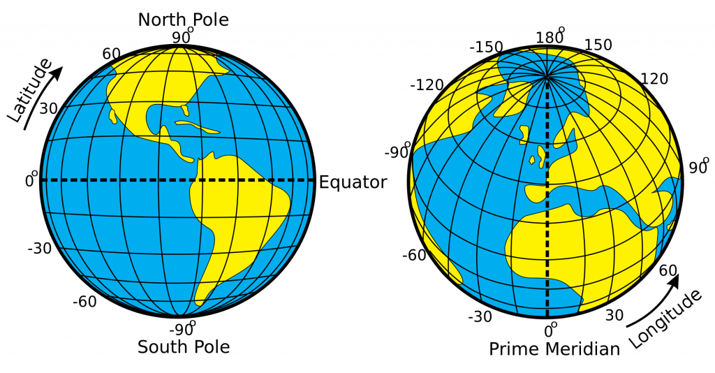
The geographical coordinate system measures location from only two values, despite the fact that the locations are described for a three-dimensional surface. The two values used to define location are both measured relative to the polar axis of the Earth. The two measures used in the geographic coordinate system are called latitude and longitude.

Latitude is an angular measurement north or south of the equator relative to a point found at the center of the Earth. This central point is also located on the Earth’s rotational or polar axis. The equator is the starting point for the measurement of latitude. The equator has a value of zero degrees. A line of latitude or parallel of 30° North has an angle that is 30° north of the plane represented by the equator. The maximum value that latitude can attain is either 90° North or South. These lines of latitude run parallel to the rotational axis of the Earth.

Lines connecting points of the same latitude, called parallels, has lines running parallel to each other. The only parallel that is also a great circle is the equator. All other parallels are small circles. The following are the most important parallel lines:

• Equator, 0 degrees
• Tropic of Cancer, 23.5 degrees N
• Tropic of Capricorn, 23.5 degrees S
• Arctic Circle, 66.5 degrees N
• Antarctic Circle, 66.5 degrees S
• North Pole, 90 degrees N (infinitely small circle)
• South Pole, 90 degrees S (infinitely small circle)

Longitude is the angular measurement east and west of the Prime Meridian. The position of the Prime Meridian was determined by international agreement to be in-line with the location of the former astronomical observatory at Greenwich, England. Because the Earth’s circumference is similar to a circle, it was decided to measure longitude in degrees. The number of degrees found in a circle is 360. The Prime Meridian has a value of zero degrees. A line of longitude or meridian of 45° West has an angle that is 45° west of the plane represented by the Prime Meridian. The maximum value that a meridian of longitude can have is 180° which is the distance halfway around a circle. This meridian is called the International Date Line. Designations of west and east are used to distinguish where a location is found relative to the Prime Meridian. For example, all of the locations in North America have a longitude that is designated west.

At 180 degrees of the Prime Meridian in the Pacific Ocean is the International Date Line. The line determines where the new day begins in the world. Now because of this, the International Date Line is not a straight line, rather it follows national borders so that a country is not divided into two separate days.

Ultimately, when parallel and meridian lines are combined, the result is a geographic grid system that allows users to determine their exact location on the planet.

This may be an appropriate time to briefly discuss the fact that the earth is round and not flat.

Great and Small Circles

Much of Earth’s grid system is based on the location of the North Pole, South Pole, and the Equator. The poles are an imaginary line running from the axis of Earth’s rotation. The plane of the equator is an imaginary horizontal line that cuts the earth into two halves. This brings up the topic of great and small circles. A great circle is any circle that divides the earth into a circumference of two halves. It is also the largest circle that can be drawn on a sphere. The line connecting any points along a great circle is also the shortest distance between those two points.

Examples of great circles include the Equator, all lines of longitude, the line that divides the earth into day and night called the circle of illumination, and the plane of the ecliptic, which divides the earth into equal halves along the equator. Small circles are circles that cut the earth, but not into equal halves.

Universal Transverse Mercator System (UTM)

Another commonly used method to describe a location on the Earth is the Universal Transverse Mercator (UTM) grid system. This rectangular coordinate system is metric, incorporating the meter as its basic unit of measurement. UTM also uses the Transverse Mercator projection system to model the Earth’s spherical surface onto a two-dimensional plane. The UTM system divides the world’s surface into 60, six-degree longitude-wide zones that run north-south. These zones start at the International Date Line and are successively numbered in an eastward direction. Each zone stretches from 84° North to 80° South. In the center of each of these zones is a central meridian.

Location is measured in these zones from a false origin, which is determined relative to the intersection of the equator and the central meridian for each zone. For locations in the Northern Hemisphere, the false origin is 500,000 meters west of the central meridian on the equator. Coordinate measurements of location in the Northern Hemisphere using the UTM system are made relative to this point in meters in eastings (longitudinal distance) and northings (latitudinal distance). The point defined by the intersection of 50° North and 9° West would have a UTM coordinate of Zone 29, 500000 meters east (E), 5538630 meters north (N). In the Southern Hemisphere, the origin is 10,000,000 meters south and 500,000 meters west of the equator and central meridian, respectively. The location found at 50° South and 9° West would have a UTM coordinate of Zone 29, 500000 meters E, 4461369 meters N (remember that northing in the Southern Hemisphere is measured from 10,000,000 meters south of the equator).

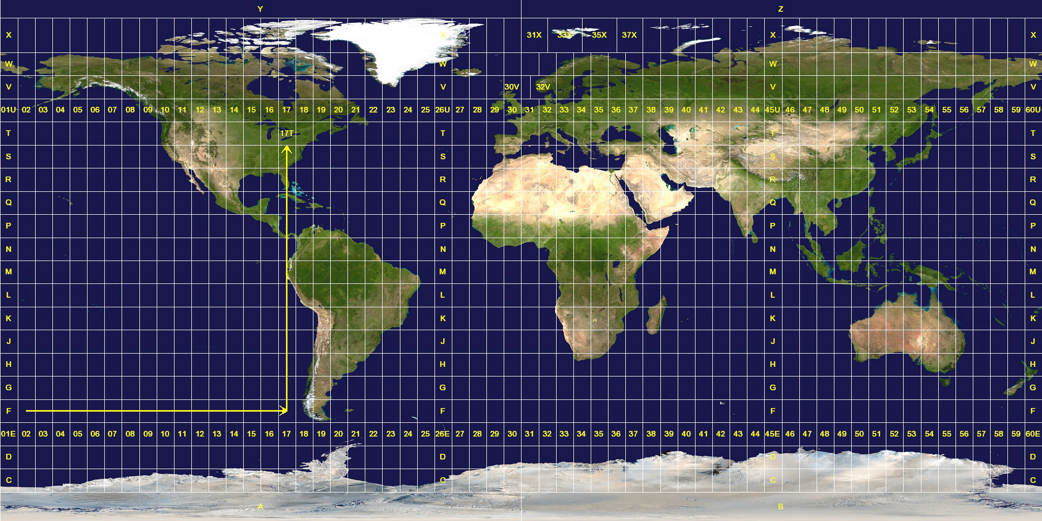
The UTM system has been modified to make measurements less confusing. In this modification, the six degree wide zones are divided into smaller pieces or quadrilaterals that are eight degrees of latitude tall. Each of these rows is labeled, starting at 80° South, with the letters C to X consecutively with I and O being omitted. The last row X differs from the other rows and extends from 72 to 84° North latitude (twelve degrees tall). Each of the quadrilaterals or grid zones are identified by their number/letter designation. In total, 1200 quadrilaterals are defined in the UTM system.

The quadrilateral system allows us to define location further using the UTM system. For the location 50° North and 9° West, the UTM coordinate can now be expressed as Grid Zone 29U, 500000 meters E, 5538630 meters N.

Each UTM quadrilateral is further subdivided into a number of 100,000 by 100,000-meter zones. These subdivisions are coded by a system of letter combinations where the same two-letter combination is not repeated within 18 degrees of latitude and longitude. Within each of the 100,000-meter squares, one can specify a location to one-meter accuracy using a five-digit eastings and northings reference system.

The UTM grid system is displayed on all United States Geological Survey (USGS) and National Topographic Series (NTS) of Canada maps. On USGS 7.5-minute quadrangle maps (1:24,000 scale), 15-minute quadrangle maps (1:50,000, 1:62,500, and standard-edition 1:63,360 scales), and Canadian 1:50,000 maps the UTM grid lines are drawn at intervals of 1,000 meters. Both are shown either with blue ticks at the edge of the map or by full blue grid lines. On USGS maps at 1:100,000 and 1:250,000 scale and Canadian 1:250,000 scale maps a full UTM grid is shown at intervals of 10,000 meters.

2.2 Time Zones

Before the late nineteenth century, timekeeping was primarily a local phenomenon. Each town would set their clocks according to the motions of the Sun. Noon was defined as the time when the Sun reached its maximum altitude above the horizon. Cities and towns would assign a clockmaker to calibrate a town clock to these solar motions. This town clock would then represent “official” time, and the citizens would set their watches and clocks accordingly.

The ladder half of the nineteenth century was a time of increased movement of humans. In the United States and Canada, large numbers of people were moving west and settlements in these areas began expanding rapidly. To support these new settlements, railroads moved people and resources between the various cities and towns. However, because of the nature of how local time was kept, the railroads experience significant problems in constructing timetables for the various stops. Timetables could only become more efficient if the towns and cities adopted some standard method of keeping time.

In 1878, Canadian Sir Sanford Fleming suggested a system of worldwide time zones that would simplify the keeping of time across the Earth. Fleming proposed that the globe should be divided into 24 time zones, every 15 degrees of longitude in width. Since the world rotates once every 24 hours on its axis and there are 360 degrees of longitude, each hour of Earth rotation represents 15 degrees of longitude.

Railroad companies in Canada and the United States began using Fleming’s time zones in 1883. In 1884, an International Prime Meridian Conference was held in Washington D.C. to adopt the standardized method of timekeeping and determined the location of the Prime Meridian. Conference members agreed that the longitude of Greenwich, England would become zero degrees longitude and established the 24 time zones relative to the Prime Meridian. It was also proposed that the measurement of time on the Earth would be made relative to the astronomical measurements at the Royal Observatory at Greenwich. This time standard was called Greenwich Mean Time (GMT).

Today, many nations operate on variations of the time zones suggested by Sir Fleming. In this system, time in the various zones is measured relative the Coordinated Universal Time (UTC) standard at the Prime Meridian. Coordinated Universal Time became the standard legal reference of time all over the world in 1972. UTC is determined from atomic clocks that are coordinated by the International Bureau of Weights and Measures (BIPM) located in France. The numbers located at the bottom of the time zone map indicate how many hours each zone is earlier (negative sign) or later (positive sign) than the Coordinated Universal Time standard. Also, note that national boundaries and political matters influence the shape of the time zone boundaries. For example, China uses a single time zone (eight hours ahead of Coordinated Universal Time) instead of five different time zones.

2.3 Coordinate Systems and Projections

Distance on Maps

Depicting the Earth’s three-dimensional surface on a two-dimensional map creates a variety of distortions that involve distance, area, and direction. It is possible to create maps that are somewhat equidistance. However, even these types of maps have some form of distance distortion. Equidistance maps can only control distortion along either lines of latitude or lines of longitude. Distance is often correct on equidistance maps only in the direction of latitude.

On a map that has a large scale, 1:125,000 or larger, distance distortion is usually insignificant. An example of a large-scale map is a standard topographic map. On these maps measuring straight line distance is simple. Distance is first measured on the map using a ruler. This measurement is then converted into a real-world distance using the map’s scale. For example, if we measured a distance of 10 centimeters on a map that had a scale of 1:10,000, we would multiply 10 (distance) by 10,000 (scale). Thus, the actual distance in the real world would be 100,000 centimeters.

Measuring distance along map features that are not straight is a little more difficult. One technique that can be employed for this task is to use several straight-line segments. The accuracy of this method is dependent on the number of straight-line segments used. Another method for measuring curvilinear map distances is to use a mechanical device called an opisometer. This device uses a small rotating wheel that records the distance traveled. The recorded distance is measured by this device either in centimeters or inches.

Direction on Maps

Like distance, direction is difficult to measure on maps because of the distortion produced by projection systems. However, this distortion is quite small on maps with scales larger than 1:125,000. Direction is usually measured relative to the location of North or South Pole. Directions determined from these locations are said to be relative to True North or True South. The magnetic poles can also be used to measure direction. However, these points on the Earth are located in spatially different spots from the geographic North and South Pole. The North Magnetic Pole is located at 78.3° North, 104.0° West near Ellef Ringnes Island, Canada. In the Southern Hemisphere, the South Magnetic Pole is located in Commonwealth Day, Antarctica and has a geographical location of 65° South, 139° East. The magnetic poles are also not fixed over time and shift their spatial position over time.

Topographic maps typically have a declination diagram drawn on them. On Northern Hemisphere maps, declination diagrams describe the angular difference between Magnetic North and True North. On the map, the angle of True North is parallel to the depicted lines of longitude. Declination diagrams also show the direction of Grid North. Grid North is an angle that is parallel to the easting lines found on the Universal Transverse Mercator (UTM) grid system.

In the field, the direction of features is often determined by a magnetic compass which measures angles relative to Magnetic North. Using the declination diagram found on a map, individuals can convert their field measures of magnetic direction into directions that are relative to either Grid or True North. Compass directions can be described by using either the azimuth system or the bearing system. The azimuth system calculates direction in degrees of a full circle. A full circle has 360 degrees. In the azimuth system, north has a direction of either the 0 or 360°. East and West have an azimuth of 90° and 270°, respectively. Due south has an azimuth of 180°.

The bearing system divides direction into four quadrants of 90 degrees. In this system, north and south are the dominant directions. Measurements are determined in degrees from one of these directions.

Geography is about spatial understanding, which requires an accurate grid system to determine absolute and relative location. Absolute location is the exact x- and y- coordinate on the Earth. Relative location is the location of something relative to other entities. For example, when someone uses his or her GPS on his or her smartphone or car, they will put in an absolute location. However, as they start driving, the device tells them to turn right or left relative to objects on the ground.

2.4 Geospatial Technology

Data, data, data… data is everywhere. There are two basic types of data to be familiar with: spatial and non-spatial data. Spatial data, also called geospatial data, is data directly related to a specific location on Earth. Geospatial data is becoming “big business” because it is not just data, but data that can be located, tracked, patterned, and modeled based on other geospatial data. Census information that is collected every ten years is an example of spatial data. Non-spatial data is data that cannot be traced to a specific location, including the number of people living in a household, enrollment within a specific course, or gender information. However, non-spatial data can easily become spatial data if it can connect in some way to a location. Geospatial technology specialists have a method called geocoding that can be used to give non-spatial data a geographic location. Once data has a spatial component associated with it, the type of questions that can be asked dramatically changes.

Remote Sensing

Remote sensing can be defined as the collection of data about an object from a distance. Humans and many other types of animals accomplish this task with the aid of eyes or by the sense of smell or hearing. Geographers use the technique of remote sensing to monitor or measure phenomena found in the Earth’s lithosphere, biosphere, hydrosphere, and atmosphere. Remote sensing of the environment by geographers is usually done with the help of mechanical devices known as remote sensors. These gadgets have a significantly improved ability to receive and record information about an object without any physical contact. Often, these sensors are positioned away from the object of interest by using helicopters, planes, and satellites. Most sensing devices record information about an object by measuring an object’s transmission of electromagnetic energy from reflecting and radiating surfaces.

Remote sensing imagery has many applications in mapping land-use and cover, agriculture, soils mapping, forestry, city planning, archaeological investigations, military observation, and geomorphological surveying, among other uses. For example, foresters use aerial photographs for preparing forest cover maps, locating possible access roads, and measuring quantities of trees harvested. Specialized photography using color infrared film has also been used to detect disease and insect damage in forest trees.

Satellite Remote Sensing

The simplest form of remote sensing uses photographic cameras to record information from visible or near-infrared wavelengths. In the late 1800s, cameras were positioned above the Earth’s surface in balloons or kites to take oblique aerial photographs of the landscape. During World War I, aerial photography played an important role in gathering information about the position and movements of enemy troops. These photographs were often taken from airplanes. After the war, civilian use of aerial photography from airplanes began with the systematic vertical imaging of large areas of Canada, the United States, and Europe. Many of these images were used to construct topographic and other types of reference maps of the natural and human-made features found on the Earth’s surface.

The development of color photography following World War II gave a more natural depiction of surface objects. Color aerial photography also substantially increased the amount of information gathered from an object. The human eye can differentiate many more shades of color than tones of gray. In 1942, Kodak developed color infrared film, which recorded wavelengths in the near-infrared part of the electromagnetic spectrum. This film type had good haze penetration and the ability to determine the type and health of vegetation.

In the 1960s, a revolution in remote sensing technology began with the deployment of space satellites. From their high vantage-point, satellites have an extended view of the Earth’s surface. The first meteorological satellite, TIROS-1, was launched by the United States using an Atlas rocket on April 1, 1960. This early weather satellite used vidicon cameras to scan broad areas of the Earth’s surface. Early satellite remote sensors did not use conventional film to produce their images. Instead, the sensors digitally capture the images using a device similar to a television camera. Once captured, this data is then transmitted electronically to receiving stations found on the Earth’s surface.

In the 1970s, the second revolution in remote sensing technology began with the deployment of the Landsat satellites. Since this 1972, several generations of Landsat satellites with their Multispectral Scanners (MSS) have been providing continuous coverage of the Earth for almost 30 years. Current, Landsat satellites orbit the Earth’s surface at an altitude of approximately 700 kilometers. The spatial resolution of objects on the ground surface is 79 x 56 meters. Complete coverage of the globe requires 233 orbits and occurs every 16 days. The Multispectral Scanner records a zone of the Earth’s surface that is 185 kilometers wide in four wavelength bands: band 4 at 0.5 to 0.6 micrometers, band 5 at 0.6 to 0.7 micrometers, band 6 at 0.7 to 0.8 micrometers, and band 7 at 0.8 to 1.1 micrometers. Bands 4 and 5 receive the green and red wavelengths in the visible light range of the electromagnetic spectrum. The last two bands image near-infrared wavelengths. A second sensing system was added to Landsat satellites launched after 1982. This imaging system, known as the Thematic Mapper, records seven wavelength bands from the visible to far-infrared portions of the electromagnetic spectrum. Also, the ground resolution of this sensor was enhanced to 30 x 20 meters. This modification allows for significantly improved clarity of imaged objects.

The usefulness of satellites for remote sensing has resulted in several other organizations launching their own devices. In France, the SPOT (Satellite Pour l’Observation de la Terre) satellite program has launched five satellites since 1986. Since 1986, SPOT satellites have produced more than 10 million images. SPOT satellites use two different sensing systems to image the planet. One sensing system produces black and white panchromatic images from the visible band (0.51 to 0.73 micrometers) with a ground resolution of 10 x 10 meters. The other sensing device is multispectral capturing green, red, and reflected infrared bands at 20 x 20 meters. SPOT-5, which was launched in 2002, is much improved from the first four versions of SPOT satellites. SPOT-5 has a maximum ground resolution of 2.5 x 2.5 meters in both panchromatic mode and multispectral operation.

Radarsat-1 was launched by the Canadian Space Agency in November, 1995. As a remote sensing device, Radarsat is entirely different from the Landsat and SPOT satellites. Radarsat is an active remote sensing system that transmits and receives microwave radiation. Landsat and SPOT sensors passively measure reflected radiation at wavelengths roughly equivalent to those detected by our eyes. Radarsat’s microwave energy penetrates clouds, rain, dust, or haze and produces images regardless of the Sun’s illumination allowing it to image in darkness. Radarsat images have a resolution between 8 to 100 meters. This sensor has found important applications in crop monitoring, defense surveillance, disaster monitoring, geologic resource mapping, sea-ice mapping and monitoring, oil slick detection, and digital elevation modeling.

Today, the GOES (Geostationary Operational Environmental Satellite) system of satellites provides most of the remotely sensed weather information for North America. To cover the entire continent and adjacent oceans, two satellites are employed in a geostationary orbit. The western half of North America and the eastern Pacific Ocean is monitored by GOES-10, which is directly above the equator and 135° West longitude. The eastern half of North America and the western Atlantic are cover by GOES-8. The GOES-8 satellite is located overhead of the equator and 75° West longitude. Advanced sensors aboard the GOES satellite produce a continuous data stream so images can be viewed at any instance. The imaging sensor produces visible and infrared images of the Earth’s terrestrial surface and oceans. Infrared images can depict weather conditions even during the night. Another sensor aboard the satellite can determine vertical temperature profiles, vertical moisture profiles, total precipitable water, and atmospheric stability.

Principles of Object Identification

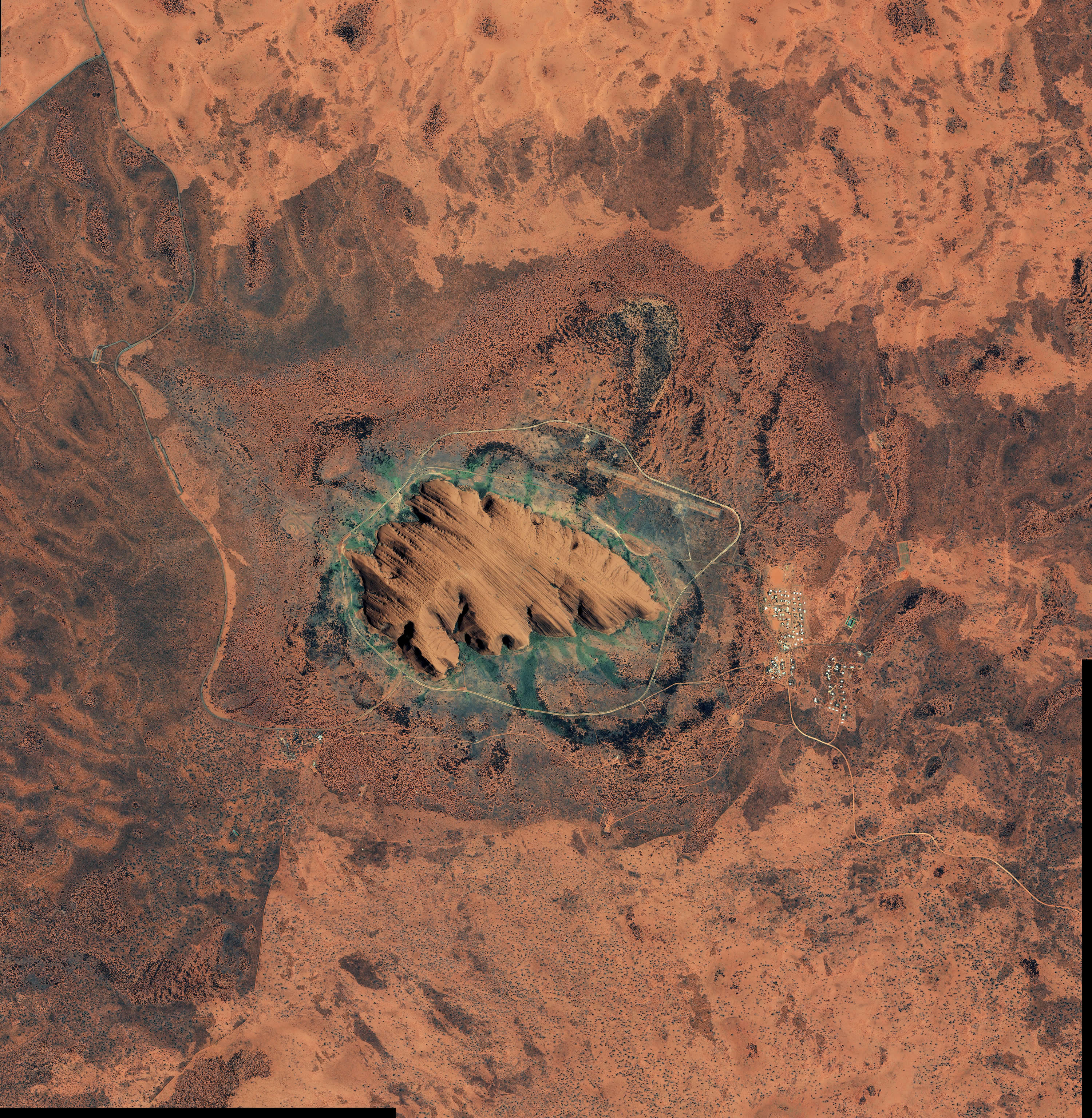
Most people have no problem identifying objects from photographs taken from an oblique angle. Such views are natural to the human eye and are part of our everyday experience. However, most remotely sensed images are taken from an overhead or vertical perspective and distances quite removed from ground level. Both of these circumstances make the interpretation of natural and human-made objects somewhat difficult. In addition, images obtained from devices that receive and capture electromagnetic wavelengths outside human vision can present views that are quite unfamiliar.

To overcome the potential difficulties involved in image recognition, professional image interpreters use some characteristics to help them identify remotely sensed objects. Some of these characteristics include:

• Shape: this characteristic alone may serve to identify many objects. Examples include the long linear lines of highways, the intersecting runways of an airfield, the perfectly rectangular shape of buildings, or the recognizable shape of an outdoor baseball diamond.
• Size: noting the relative and absolute sizes of objects are essential in their identification. The scale of the image determines the absolute size of an object. As a result, it is essential to recognize the scale of the image to be analyzed.
• Image Tone or Color: all objects reflect or emit specific signatures of electromagnetic radiation. In most cases, related types of objects emit or reflect similar wavelengths of radiation. Also, the types of the recording device and recording media produce images that are reflective of their sensitivity to a particular range of radiation. As a result, the interpreter must be aware of how the object being viewed will appear on the image examined. For example, on color, infrared images vegetation has a color that ranges from pink to red rather than the usual tones of green.
• Pattern: many objects arrange themselves in typical patterns. This is especially true of human-made phenomena. For example, orchards have a systematic arrangement imposed by a farmer, while natural vegetation usually has a random or chaotic pattern.
• Shadow: shadows can sometimes be used to get a different view of an object. For example, an overhead photograph of a towering smokestack or a radio transmission tower normally presents an identification problem. This difficulty can be overcome by photographing these objects at Sun angles that cast shadows. These shadows then display the shape of the object on the ground. Shadows can also be a problem to interpreters because they often conceal things found on the Earth’s surface.
• Texture: imaged objects display some degree of coarseness or smoothness. This characteristic can sometimes be useful in object interpretation. For example, we would typically expect to see textural differences when comparing an area of grass with field corn. Texture, just like object size, is directly related to the scale of the image.

Global Positioning Systems

Another type of geospatial technology is global positioning systems (GPS) and a key technology for acquiring accurate control points on Earth’s surface. Now to determine the location of that GPS receiver on Earth’s surface, a minimum of four satellites is required using a mathematical process called triangulation. Usually, the process of triangulation requires a minimum of three transmitters, but because the energy sent from the satellite is traveling at the speed of light, minor errors in calculation could result in significant location errors on the ground. Thus, a minimum of four satellites is often used to reduce this error. This process using the geometry of triangles to determine location is used not only in GPS, but a variety of other location needs like finding the epicenter of earthquakes.

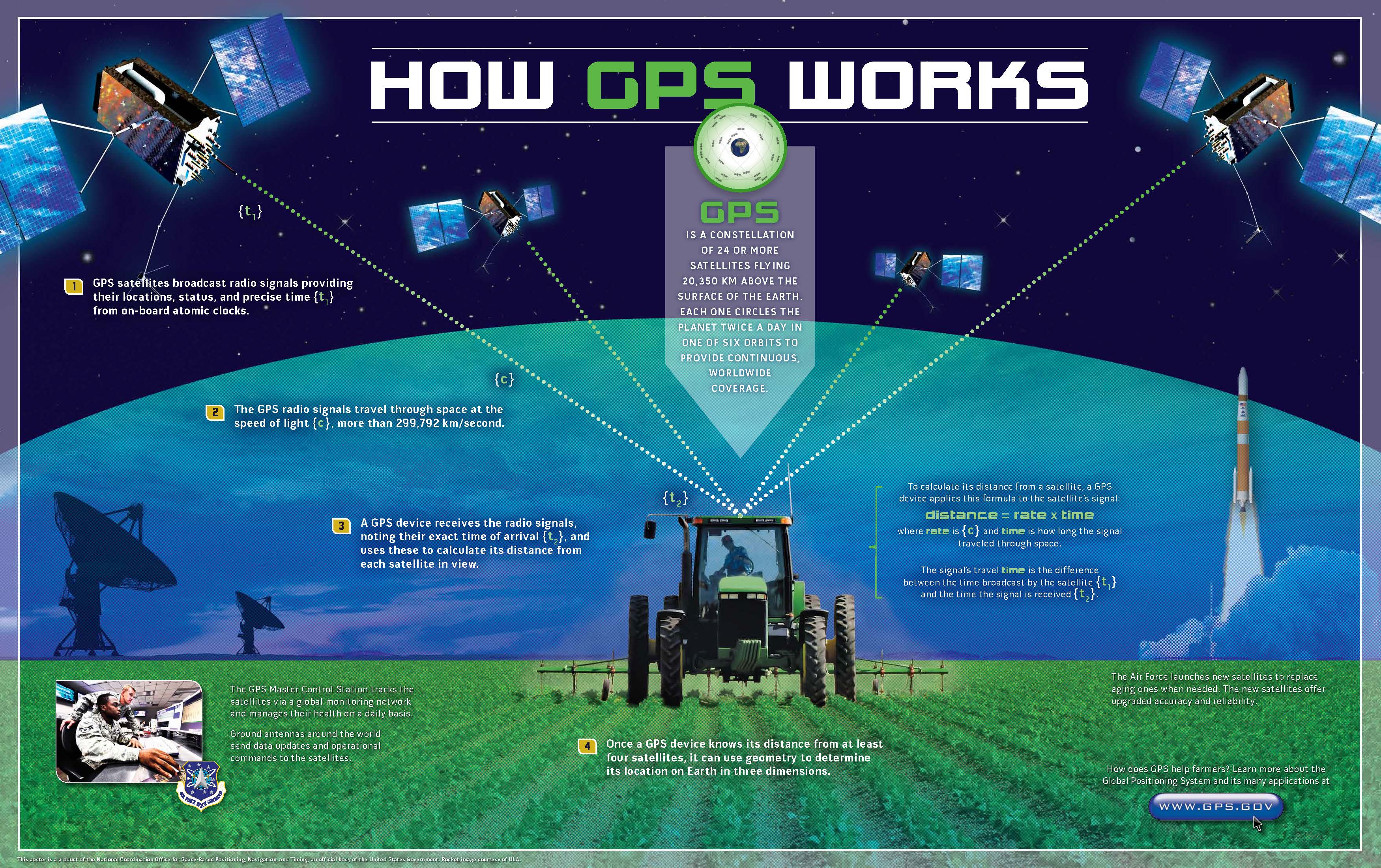
A user can use a GPS receiver to determine their location on Earth through a dynamic conversation with satellites in space. Each satellite transmits orbital information called the ephemeris using a highly accurate atomic clock along with its orbital position called the almanac. The receiver will use this information to determine its distance from a single satellite using the equation D = rt, where D = distance, r = rate or the speed of light (299,792,458 meters per second), and t = time using the atomic clock. The atomic clock is required because the receiver is trying to calculate distance, using energy that is transmitted at the speed of light. Time will be fractions of a second and requires a “time clock” up the utmost accuracy.

Determination of location in field conditions was once a difficult task. In most cases, it required the use of a topographic map and landscape features to estimate location. However, technology has now made this task very simple. Global Positioning Systems (GPS) can calculate one’s location to an accuracy of about 30-meters. These systems consist of two parts: a GPS receiver and a network of many satellites. Radio transmissions from the satellites are broadcasted continually. The GPS receiver picks up these broadcasts and through triangulation calculates the altitude and spatial position of the receiving unit. A minimum of three satellite is required for triangulation.

GPS receivers can determine latitude, longitude, and elevation anywhere on or above the Earth’s surface from signals transmitted by a number of satellites. These units can also be used to determine direction, distance traveled, and determine routes of travel in field situations.

Geographic Information Systems

The advent of cheap and powerful computers over the last few decades has allowed for the development of innovative software applications for the storage, analysis, and display of geographic data. Many of these applications belong to a group of software known as Geographic Information Systems (GIS). Many definitions have been proposed for what constitutes a GIS. Each of these definitions conforms to the particular task that is being performed. A GIS does the following activities:

• Measurement of natural and human-made phenomena and processes from a spatial perspective. These measurements emphasize three types of properties commonly associated with these types of systems: elements, attributes, and relationships.
• Storage of measurements in digital form in a computer database. These measurements are often linked to features on a digital map. The features can be of three types: points, lines, or areas (polygons).
• Analysis of collected measurements to produce more data and to discover new relationships by numerically manipulating and modeling different pieces of data.
• Depiction of the measured or analyzed data in some type of display – maps, graphs, lists, or summary statistics.

The first computerized GIS began its life in 1964 as a project of the Rehabilitation and Development Agency Program within the government of Canada. The Canada Geographic Information System (CGIS) was designed to analyze Canada’s national land inventory data to aid in the development of land for agriculture. The CGIS project was completed in 1971, and the software is still in use today. The CGIS project also involved a number of key innovations that have found their way into the feature set of many subsequent software developments.

From the mid-1960s to 1970s, developments in GIS were mainly occurring at government agencies and universities. In 1964, Howard Fisher established the Harvard Lab for Computer Graphics where many of the industries early leaders studied. The Harvard Lab produced a number of mainframe GIS applications including SYMAP (Synagraphic Mapping System), CALFORM, SYMVU, GRID, POLYVRT, and ODYSSEY. ODYSSEY was first modern vector GIS, and many of its features would form the basis for future commercial applications. Automatic Mapping System was developed by the United States Central Intelligence Agency (CIA) in the late 1960s. This project then spawned the CIA’s World Data Bank, a collection of coastlines, rivers, and political boundaries, and the CAM software package that created maps at different scales from this data. This development was one of the first systematic map databases. In 1969, Jack Dangermond, who studied at the Harvard Lab for Computer Graphics, co-founded Environmental Systems Research Institute (ESRI) with his wife, Laura. ESRI would become in a few years the dominant force in the GIS marketplace and create ArcInfo and ArcView software. The first conference dealing with GIS took place in 1970 and was organized by Roger Tomlinson (key individual in the development of CGIS) and Duane Marble (professor at Northwestern University and early GIS innovator). Today, numerous conferences dealing with GIS run every year attracting thousands of attendants.

In the 1980s and 1990s, many GIS applications underwent substantial evolution regarding features and analysis power. Many of these packages were being refined by private companies who could see the future commercial potential of this software. Some of the popular commercial applications launched during this period include ArcInfo, ArcView, MapInfo, SPANS GIS, PAMAP GIS, INTERGRAPH, and SMALLWORLD. It was also during this period that many GIS applications moved from expensive minicomputer workstations to personal computer hardware.

There is a technology that exists that can bring together remote sensing data, GPS data points, spatial and non-spatial data, and spatial statistics into a single, dynamic system for analysis and that is a geographic information system (GIS). A GIS is a powerful database system that allows users to acquire, organize, store, and most importantly analyze information about the physical and cultural environments. A GIS views the world as overlaying physical or cultural layers, each with quantifiable data that can be analyzed. A single GIS map of a national forest could have layers such as elevation, deciduous trees, evergreens, soil type, soil erosion rates, rivers and tributaries, major and minor roads, forest health, burn areas, regrowth, restoration, animal species type, trails, and more. Each of these layers would contain a database of information specific to that layer.

GIS combines computer cartography with a database management system. GIS consists of three subsystems: (1) an input system that allows for the collection of data to be used and analyzed for some purpose; (2) computer hardware and software systems that store the data, allow for data management and analysis, and can be used to display data manipulations on a computer monitor; (3) an output system that generates hard copy maps, images, and other types of output.

Two basic types of data are typically entered into a GIS. The first type of data consists of real-world phenomena and features that have some form of spatial dimension. Usually, these data elements are depicted mathematically in the GIS as either points, lines, or polygons that are referenced geographically (or geocoded) to some type of coordinate system. This type data is entered into the GIS by devices like scanners, digitizers, GPS, air photos, and satellite imagery. The other type of data is sometimes referred to as an attribute. Attributes are pieces of data that are connected or related to the points, lines, or polygons mapped in the GIS. This attribute data can be analyzed to determine patterns of importance. Attribute data is entered directly into a database where it is associated with feature data.

Within the GIS database, a user can enter, analyze, and manipulate data that is associated with some spatial element in the real world. The cartographic software of the GIS enables one to display the geographic information at any scale or projection and as a variety of layers which can be turned on or off. Each layer would show some different aspect of a place on the Earth. These layers could show things like a road network, topography, vegetation cover, streams and water bodies, or the distribution of annual precipitation received.

Nearly every discipline, career path, or academic pursuit uses geographic information systems because of the vast amount of data and information about the physical and cultural world. Disciplines and career paths that use GIS include: conservation, ecology, disaster response and mitigation, business, marketing, engineering, sociology, demography, astronomy, transportation, health, criminal justice and law enforcement, travel and tourism, news media, and the list could endlessly go on.

Now, GIS primarily works from two different spatial models: raster and vector. Raster models in GIS are images much like a digital picture. Each image is broken down into a series of columns and rows of pixels, and each pixel is georeferenced to somewhere on Earth’s surface is represents a specific numeric value – usually a specific color or wavelength within the electromagnetic spectrum. Most remote sensing images come into a GIS as a raster layer.

The other type of GIS model is called a vector model. Vector-based GIS models are based on the concept of points that are again georeferenced (i.e., given an x-, y-, and possibly z- location) to somewhere specific on the ground. From points, lines can be created by connecting a series of points and areas can be created by closing loops of vector lines. For each of these vector layers, a database of information can be attributed to it. So for example, a vector line of rivers could have a database associated with it such as length, width, stream flow, government agencies responsible for it, and anything else the GIS user wants to be connected to it. What these vector models represent is also a matter of scale. For example, a city can be represented as a point or a polygon depending on how zoomed in you are to the location. A map of the world would show cities as points, whereas a map of a single county may show the city as a polygon with roads, populations, pipes, or grid systems within it.

References

This work is licensed under a Creative Commons Attribution 4.0 International License.