
Fantastic Exoplanets and Where to Find Them
Download a pdf of this paper
Joseph Hinchey, Howard Community College
William Jeffreys, Howard Community College
Parsa Samadani, Howard Community College
Mentored by: Brendan Diamond, Ph.D.
Abstract
An exoplanet is any planet outside of our solar system, and our research team wanted to demonstrate that Howard Community College (HCC) has the ability to detect them. By observing the drop in a host star’s brightness as an exoplanet orbits around it and in front of our field of view, the exoplanet’s size and inclination can be determined with some prior knowledge about its host star. A 14” telescope was assembled and used on HCC’s campus to take a sequence of images before, during, and after the predicted transit. A known exoplanet was selected with a promising predicted transit to measure its properties and demonstrate the capability of the new equipment. Data is presented from a successfully observed transit on November 4th, 2018 of exoplanet WASP-50b around the host star WASP-50. During the 1.8-hour transit, a 1.6% (±0.1%) drop in brightness was observed in the host star. Inputting the change in brightness over time into an accepted model, we inferred the existence of an exoplanet with a diameter 15% (±1%) larger than Jupiter and an inclination of 86° (±2°), which is consistent with published values. The long-term goal of the project is to contribute to the field of astronomy through collaboration with the recently-launched Transiting Exoplanet Survey Satellite (TESS).
Introduction
As humans, one of the natural qualities that helps define us is our passionate curiosity for exploring the universe and the ability to create tools to help aid us in this quest. One of humanity’s greatest frontiers, when it comes to exploring the unknown, is space. To one day explore exoplanets (planets beyond our own solar system) would be an incredible feat. However, this is a complicated goal that would be difficult to achieve without first observing the very worlds that we dream of reaching. The very first exoplanet was found in 1995 and as of today, there are about 4000 exoplanets that have been found using various methods. Some of these methods include, but are not limited to, radial velocity, microlensing, and using transit photometry. Radial velocity was once the most effective and common method for locating exoplanets until the planet hunting space telescope, Kepler, was launched in 2009. Kepler utilized transit photometry to search for exoplanets [1]. Now, with the transit method, even amateur level telescopes can detect evidence of exoplanets [2].
Our research team wanted to test the group’s ability to detect evidence supporting the existence of exoplanets with equipment at Howard Community College and potentially participate in future related research with the NASA’s Transiting Exoplanet Survey Satellite (TESS). TESS’s mission is to take images over the entire sky, looking for temporary dips in brightness of the stars to locate possible locations for exoplanet. These images are then available to astronomers, allowing to analyze small sections of the complete survey in order to confirm the existence of potential exoplanets [3]. As can be seen in Figure 1, the transit method detects the dimming of the star’s light as an orbiting exoplanet passes between it and the Earth.
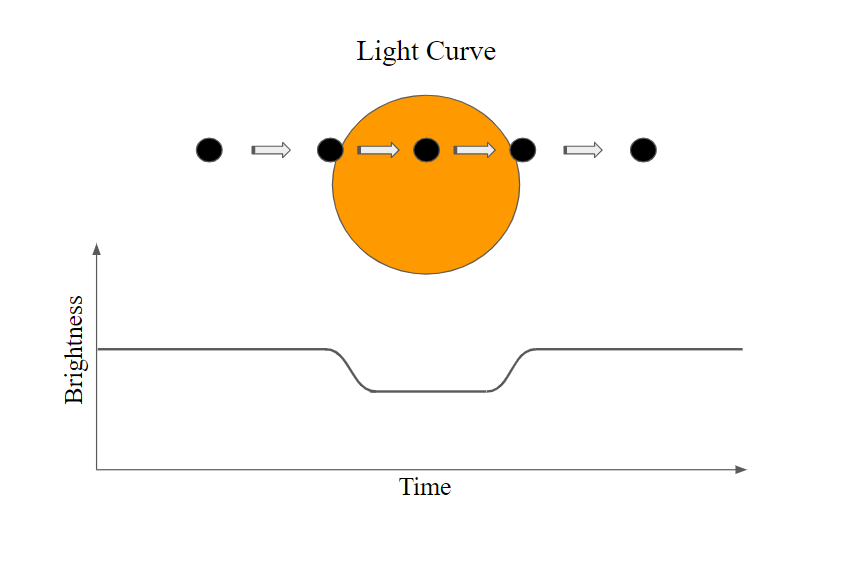
Figure 1: A light curve is a representation of how the detected brightness of the star changes during a transit. The detected brightness of
the star decreases while the exoplanet blocks a small portion of the light emitted by the star.
Equipment and Software
Throughout the course of our research and planning, we utilized a few specialized pieces of equipment that the college purchased in conjunction with the new Science Engineering and Technology building. The set of equipment we used, shown in Figure 2, are comprised of a 14” PlaneWave telescope, an AstroPhysics 1100gto equatorial mount and an SBIG STXL-6303E camera. An equatorial mount has a motor aligned with rotation axis of the earth to counteract the earth’s rotation making it possible for the telescope to precisely follow the star. The software used for capturing images was MaxIm DL [4] and image processing and data analysis was done with AstroImageJ software [5]. The mount, telescope, and camera were all assembled on-site atop the observation deck of HCC’s Science Engineering & Technology building. Over the course of about two months and approximately 15 hours of total build time, we assembled the components as they were shipped to us. With a protective outdoor cover, the entire unit is now available for use whenever is necessary and can be stored indoors during extended breaks.
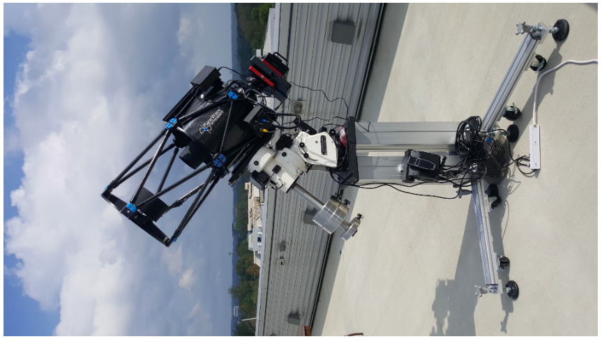
Figure 2: 14” PlaneWave telescope, AstroPhysics 1100gto equatorial mount, and SBIG STXL-6303E camera assembled and used in the fall of 2018 at Howard Community College.
Obtaining Images
To begin the process of gathering our collection of images to reduce, we first had to decide on a target star that we thought would result in clear, distinguishable data. We used a website, “Find Exoplanet Transits”, developed by Swarthmore College to look at a list of stars known to host exoplanets with transits in the coming days visible from our location (39° 12′ 53.32” N, 76° 52′ 52.38” W) [6]. There were specific qualities we searched for that would make a star a good candidate for observation. Qualities such as a low magnitude, a large projected depth, an altitude >10°. A lower magnitude means a star is brighter so it’s not challenging to locate the star. A large projected depth (in milli-magnitude) for the transit is preferred so the changes in brightness are more apparent. An altitude >10° would be far enough from the horizon resulting in less atmospheric interference. After several unsuccessful attempts at observing due to calibration issues, technical problems, and tracking issues, we had a successful observation November 4th, 2018. The target star that evening was WASP-50, with a magnitude of 11.60, a predicted depth of 21.2 m-mag, and an altitude at mid-transit of 37.6° [6].
The exoplanet in our study, named WASP-50b, had a total predicted transit time of about 1 hour and 48 minutes, lasting from 12:48am to 1:36am local time on the night of November 3rd_4th (coinciding with the change for daylight saving time). The standard for naming exoplanets is simply adding a letter to the end of the host star name. We began preparing for the observation the evening of November 3rd by setting the filter wheel to use an Astrodon Exoplanet filter and making sure the telescope was properly aligned and all equipment was working properly. In order to capture a noticeable drop in light from the star, we needed to allow time to receive its normal light output before the transit, meaning we would have to begin collecting images at 12:00am_12:10am (about 30 minutes before the transit). A number of the accepted values that had been calculated and measured on WASP-50, from the literature, are included in Table 1.
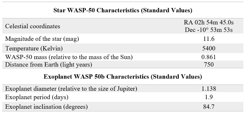
Table 1: The properties and accepted values of WASP-50 and its exoplanet [7] related to our ability to measure the effect of the exoplanet on star’s brightness.
The locating process was fairly quick this time, as we had practiced for a handful of long nights prior. We began by using the given coordinates of WASP-50 and inputting them into the telescope’s control board, which slewed us to the general area of the sky that it resided. Then, in order to determine which star was WASP-50 out of the dozens that were in our view, we opened up a celestial map [8] around our target star (WASP-50) and looked for any star patterns we could recognize [9]. Once WASP-50 was located, the telescope mount was set to track it and take 90 second exposures over the course of about 2 hours at a constant camera temperature of -15 ℃. The star did drift across the image during the transit, contributing to the variation in brightness. The exposure time of 90 seconds was chosen by testing several exposures and selecting the shortest time that gave a sufficient amount of light on each pixel, to ensure a linear relationship between the light striking the sensor and the electrical current generated as a result.
Calibration images were obtained after the science images or “lights” (images of stars), were completed. We began collecting calibration images by taking dark images (darks) by doing fifteen 90-second exposures with the charged-coupled device (CCD aka camera) shutter closed. The completely dark images allow us to detect and remove any defective pixels that could be mistaken as stars or otherwise interfere with measurements. Then we took flat images (flats) by imaging an Aurora Flatfield Panel (a type of uniform white light) fifteen times with one-second exposures. This gave us an almost completely white image, allowing us to scale the maximum pixel brightness of the CCD and reduce the impact of dust on any optical components. This removed the effect of any dust particles that might have been present on the camera lens while taking the science images. Then, we concluded our data collection for that night by taking 25 bias images (bias), which are zero second exposures to purely capture the electronic noise from the CCD and remove it from the science images as well.
Data Reduction
After all necessary images were taken by our telescope and camera, we used the AstroImageJ software to calibrate the science images and align them, so that the stars are in the same position in each image to account for any imprecise tracking. We then selected the comparison stars, appropriate apertures and annulus; dividers to separate the star’s light from other parts of the image in order to graph our data and model a curve. As seen in Figure 4, each of the chosen stars have three circles around them called apertures. The inner aperture is used to calculate the star’s brightness (source count) and must be set based on the size of the star so it is around the actual star (R1). The region between the outer two circles (R2-R3) is set outside but near the width of the star and gets subtracted from the star’s brightness to account for the sky background (Equation 1). We minimized the chances for a conflicting transit in our control by selecting multiple comparison stars. Since we knew that our target star would have a change in its light output as the exoplanet orbits in front of it, we had to get the data for other stars similar to our target star (shown in Figure 3) in apparent size and magnitude to make sure that the difference in light was, in fact, a result of an exoplanet and not from our equipment or other sources. To accomplish this, the AstroImageJ software uses these three apertures to measure the relative flux (brightness) of the target star compared to the comparison stars and the background. AstroImageJ then graphs the data including the light curve for our target star and the flux of the comparison stars, using the science images as the only inputs.
[latex]{\rm Relative~Flux~of~Target} = \frac{{\rm Target's-Sky~Background}}{{\rm Sum~of~Comparison~Stars'~Source~Count-Sky~Background}}[/latex]
[latex]{\rm Calibrated~Images} = \frac{\rm{(Lights - Bias - Darks)}}{{\rm Flats}}[/latex]
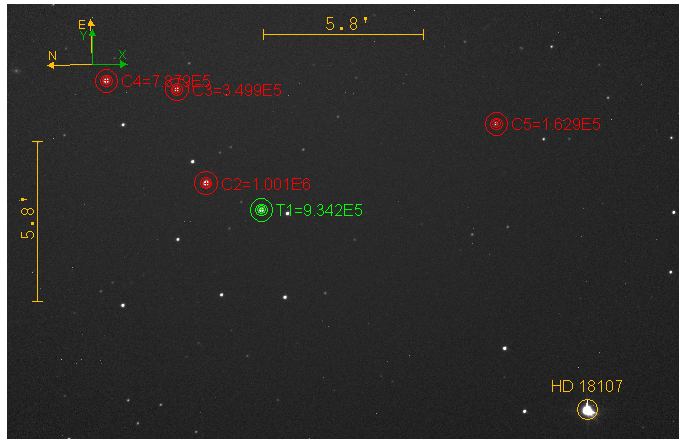
Figure 3: An image taken by our PlaneWave 14” telescope and loaded into the AstroImageJ software that shows our target star (green circle). East is up, and North is to the left in the image. The T1 circle (green) shows our target star, which is the star (WASP-50) that hosts an exoplanet. The C1-C5 circles (red) are the comparison stars, which are similar in apparent size and magnitude to our target star, to act as controls for the flux we received.
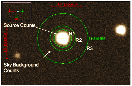
Figure 4: The rings separate different parts of the focus area to be processed for a better interpretation of the data. The inner circle (R1) is the approximate size of the star in pixels and is called the radius. The region from the radius to the middle circle (R2) accounts for any “excess” light shining outside of the star’s area. The region from the middle circle to the outer circle (R3) known as the annulus, defines what brightness the background sky is in the image. The star displayed in the center is Wasp-50, our target.
Results and Discussions
Figure 5 suggests that our target star, WASP-50, is host to an exoplanet. The exoplanet took about 1.8 hours (x-axis) to orbit in front of the star and as it did so, a small portion of the star was blocked causing a decrease of brightness (y-axis) of the star by 1.6% (±0.1). This percentage in normalized flux corresponds to a decrease of 0.016 flux in the light curve graph. The software, AstroImageJ, calculated the flux of each star similar to what’s used in equation 1 (see Data Reduction section). The data also show one extraneous point at about 0.75 days, where upon inspection of the corresponding image, it seemed that the scope experienced a temporary vibration that caused that exposure to smear. Further precision could be obtained by detrending the data to account for the change in airmass, however the impact is mitigated because the target star was near the zenith throughout the transit.
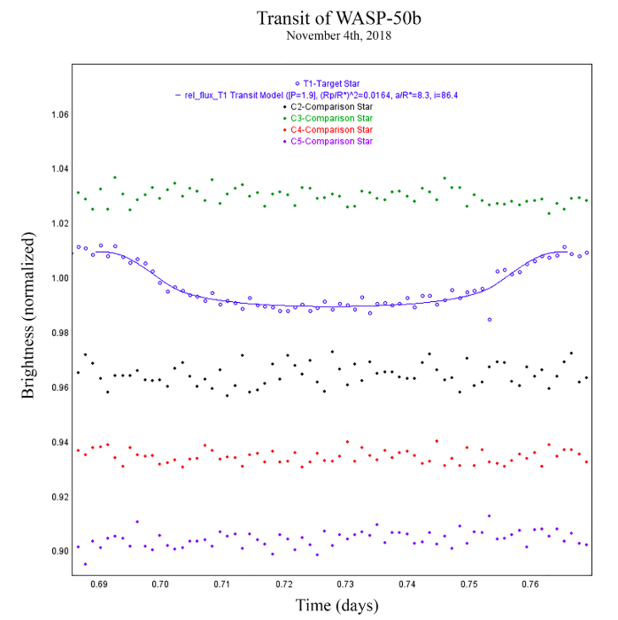
Figure 5: The brightness of the target and comparison stars in each of the images from our observation night on Nov 4th, 2018. The target star (open blue circles) is shown with a model fit and all other points represent the comparison stars. Initially all the points were at a similar normalized brightness level (~1.00) as the target star, however for clarity the comparison stars in the graph were shifted up and down.
From Figure 5 we can estimate the radius of the exoplanet using the host star’s diameter which is known from the stellar spectra to be 85.5% of our Sun’s diameter [7]. This calculation only considers the difference in brightness (D ) when the exoplanet is fully on the disk of the star. Consider,
[latex]A_p = (R_p)^2\pi[/latex]
[latex]A_s = (R_s)^2\pi[/latex]
Where [latex]A[/latex] is area, [latex]R[/latex] is radius, subscript [latex]s[/latex] is the host star, and subscript [latex]p[/latex] is the exoplanet.
[latex]\frac{A_p}{A_s} = \frac{\pi(R_p)^2}{\pi(R_s)^2} = \Delta{\rm Flux~of~Target}[/latex]
[latex]R_s = (0.855)(R_{Sun})[/latex]
[latex]\Delta{\rm Flux~of~Target} = \frac{(R_p)^2}{[(0.855)(R_{Sun})]^2}[/latex]
For convenience, we can contrast the exoplanet’s size with that of Jupiter by rewriting in terms of Jupiter’s radius,
[latex]\frac{R_{Sun}}{R_{Jupiter}} = \frac{695700~{\rm km}}{69900~{\rm km}}[/latex]
[latex]R_{Sun} = 9.95R_{Jupiter}[/latex]
Therefore, estimating our change in flux from Figure 5 to be [latex]\Delta{\rm Flux~of~Target}=0.02[/latex],
[latex]R_p \approx 1.2R_{Jupiter}[/latex]
This calculation gives us a rough estimate of the exoplanet’s size being about 20% larger than Jupiter in radius, but a more precise radius and further information about the exoplanet can be obtained using a more complex mathematical form accounting for variables such as limb darkening and orbital inclination [10]. To obtain more detailed and precise exoplanet parameters using this model to fit our data, we input the known stellar diameter of WASP-50 (0.855), the period of orbit (1.9), and the default quadratic limb darkening coefficient (0.3). Other parameters were allowed to be adjusted for a best fit by the software AstroImageJ. A best fit for the transit parameters gave an inclination of 86 (±2) degrees. Uncertainties in our measurements were estimated by running the analysis with possible stellar temperatures and radii. By comparing the exoplanet diameter, and inclination in the accepted values in Table 1 and our experimental values in Table 2, we have evidence that our results were successful because of the similarity to the accepted values measured by professional astronomers.
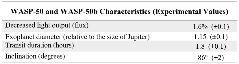
Table 2: The calculated values of WASP-50 and the observed exoplanet, WASP-50b from our observation.
Conclusion
With the results gathered from our measurements of this first transit, using the specialized equipment at HCC, we feel as though we have demonstrated that the college and its students have the capability to detect evidence of exoplanets. By refining the skills needed to detect exoplanet transits, we hope to achieve the precision and consistency needed to perform follow-up observations for international collaborations, such as TESS [3]. This was the first of many steps to participate in future research seeking to contribute more knowledge to the field of astronomy.
Acknowledgements
Thank you to Dr. Conti and Kenny A. Diazeguigure, for helping us many times throughout the semester with their expertise on equipment and exoplanets. Thanks also to Dr. Tiara Diamond for editing assistance. We would also like to thank the National Science Foundation for supporting our research with grant #1458149.
Contact: joseph.hinchey@howardcc.edu, william.jeffreys@howardcc.edu, psamadani@howardcc.edu, bdiamond@howardcc.edu
References
[1] The Planetary Society, “How to Search for Exoplanets,” [Online]. Available: http://www.planetary.org/explore/space-topics/exoplanets/how-to-search-for-exoplanets.html. [Accessed 2018].
[2] Conti, “AstroDennis,” [Online]. Available: AstroDennis.com. [Accessed 2018].
[3] R. Ricker, J. N. Winn, R. Vanderspek, D. W. Latham, G. Á. Bakos, J. L. Bean, Z. K. Berta-Thompson, T. M. Brown, L. Buchhave, N. R. Butler, R. P. Butler, W. J. Chaplin, D. Charbonneau and Chr, “Transiting Exoplanet Survey Satellite (TESS),” Proceedings of the SPIE, vol. 9143, no. 914320, p. 15, 2014.
[4] Diffraction Limited, “Getting Started,” [Online]. Available: http://diffractionlimited.com/downloads/GettingStarted.pdf. [Accessed 2018].
[5] Cornell University, “AstroImageJ: Image Processing and Photometric Extraction for Ultra-Precise Astronomical Light Curves (Expanded Edition),” [Online]. Available: https://arxiv.org/abs/1701.04817. [Accessed 2018].
[6] Swarthmore College, “Find Exoplanet Transits,” [Online]. Available: https://astro.swarthmore.edu/transits.cgi. [Accessed 2018].
[7] eu, “Planet WASP-50 b,” [Online]. Available: http://exoplanet.eu/catalog/wasp-50_b/. [Accessed 2018].
[8] CDS, “Aladin Lite,” [Online]. Available: https://aladin.u-strasbg.fr/AladinLite/. [Accessed 2018].
[9] Bonnarel, P. Fernique, O. Bieneymé, D. Egret, F. Genova, M. Louys, F. Ochsenbein, M. Wenger and J. G. Barlett, “The ALADIN interactive sky atlas. A reference tool for identification of astronomical sources,” Astronomy and Astrophysics Supplement, vol. 143, pp. 33-40, 2000.
[10] Cornell University, “Analytic Lightcurves for Planetary Transit Searches,” [Online]. Available: https://arxiv.org/abs/astro-ph/0210099. [Accessed 2018].
[11] Lang, D. Hogg, K. Mierle, M. Blanton and S. Roweis, “Astrometry.net: Blind Astrometric Calibration of Arbitrary Astronomical Images,” The Astronomical Journal, vol. 139, no. 5, pp. 1782-1800, 2010.
[12] Han, S. X. Wang, J. T. Wright, Y. K. Feng, M. Zhao, O. Fakhouri, J. I. Brown and C. Hancock, “Exoplanet Orbit Database. II. Updates to Exoplanets.org,” Publications of the Astronomical Society of the Pacific, vol. 126, no. 943, p. 827, 2014.
[13] Schneider, C. Dedieu, P. Le Sidaner, R. Savalle and I. Zolotukhin, “Defining and cataloging exoplanets: the exoplanet.eu database,” Astronomy & Astrophysics, vol. 532, no. A79, p. 11, 2011.
[14] Romanishin, “An Introduction to Astronomical Photometry Using CCDs,” 22 October 2006. [Online]. Available: http://www.physics.csbsju.edu/370/photometry/manuals/OU.edu_CCD_photometry_wrccd06.pdf. [Accessed 28 February 2019].
