
2 Building a Mathematical Model for Equestrian Show Jumping
Amy Germain, University of Wisconsin-Madison, George Washington University,
Howard Community College, Mount St. Mary’s University
Mentored by: Mike Long, Ed.D., Loretta FitzGerald Tokoly, Ph.D., & Kristel Ehrhardt
Abstract
Mathematical modeling is useful for a variety of different data sets. This article will explore applying it to the field of equestrian show jumping. The main goal is to attempt to predict competitor rankings at the highest level of global competition. The main data set for this mathematical analysis encompasses the characteristics of competitors at ten 2019 European World Cup show jumping events [7].
Based on an initial examination of the data to determine correlations between rankings and characteristic, scatterplots were created comparing the likely main contributing factors to winning. The graphs compared ranking results to jump heights, horse/rider number of competitions, competition frequency, and the horse’s age. Linear regression analysis was applied to these factors and total horse/rider competitions and rider age to find contributing factors. Linear Algebra was used with five of these factors to create a model for prediction. The equations found from the calculations of the 2019 data were used to examine 2018 data to see if the patterns or coefficients were still valid. The model was a useful estimation tool for some performances in 2019, but the model proved to be ineffective when matched to 2018 data [7].
Background
Equestrian sports can be a very mathematically-rich field. Initial research resulted in the following findings. An interesting physics study discussed horse take-off angle (40-45 degrees for a 63-inch fence), rider and horse weight (1,100 pounds for the studied horse), length of the jump (15.7 feet including the width of the jump), height of the jump (63 inches/5 feet 3 inches), the horse’s approach speed (8.3 mph) and how long the horse and rider are in the air (0.7 seconds) [1]. Another curious study discussed how the surface area of a horse can be modeled with integrals using Calculus [2]. There exists some scholarly research on performance analysis and certain factors of international showjumpers, but from a review of these abstracts (what was available), it appeared the authors focused more on horse physiology and types of faults as they related to individual jump characteristics (combination fences versus water jumps, etc.) [3,4]. These articles were reviewed to examine existing research in the field, but were not used for the mathematical analysis below.
There is a significant amount of mathematics that goes into both the design and execution of a show jumping course. Jumps need to be designed proportionally for the horse’s physical ability and vision so that the horse can accurately judge if it is an obstacle it can clear; if not it will refuse, which means abruptly halting or stepping sideways. Riders review the course in advance of the competition. They walk a course prior to riding it using an estimated length for the human stride as a measurement so that they can count the horse strides needed in between jumps, as explained visually in Figure 1 [5]. During the round, the horse and rider need to calculate various elements of the course to avoid knocking down a pole and to be able to complete the course under the time allotted to avoid a time fault. They can also incur a touch fault for the horse clipping its hooves on the top pole but not knocking it down. These elements include the number of strides, a straight or angular approach to the jump, the gait of the horse in between jumps, the sharpness of the turn to aim at a jump, and how centered the jump is on the pole [14]. Horses can even be trained to take the jump at a non-perpendicular angle with an experienced rider [6].

Data
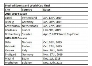
This study was conducted using event statistics from the database of the Federation Equestre Internationale (FEI), the world governing body for equestrian sports [7,8]. A sampling of ten European World Cup competitions was randomly selected from 2019, with 2018 competitions selected for comparison purposes. The competitions were from the CSI5* level, which are the World Cup competitions with the highest winnings ($177,000-$270,000 in total winnings based on the location). The competition field for each event ranged from 31-38 competitors, and some horses and riders were found in multiple events, with each performance from each event being counted as one. The size of this study was 355 performances researched for 2018 and 334 performances researched for 2019; performances were entered into an Excel spreadsheet for further study. Due to time restrictions for this study, all 2019 competitions were not examined, given there were a total of 102 global and 27 European competitions that year. The studied events, listed below in Table 1, spanned two different seasons, 2018-2019 and 2019-2020. Each World Cup series season runs from fall to spring with a final culminating World Cup event in April. Revenue for the events is collected through entry fees ($550-670 per horse) and spectator tickets. Only one or two of the events allowed betting [7].
Factors Excluded from Further Study
Certain things that could not be examined in greater detail due to a lack of information include arena material, the course design and number of jumps, and horse birthplace [7]. Factors examined that were not deemed practically significant to include in the study included final scores (not comparable across the field due to successful first-round riders engaging in a second-round “jump-off” and keeping that score), weather (competitions held in indoor arenas with stabling that may or may not be climate-controlled), horse breeds, the owner nationality, the nation the rider was competing for, and the rider’s status as an athlete, owner, official, and/or trainer (which were all varied across the competition field with no clear trend) [7,14]. A factor examined numerically that did not seem to contribute to the overall outcome included whether home country competitors are favored in a competition, which is difficult to determine in a sport where scoring is determined by time and obvious faults such as knocking down a pole [7].
Linear Regression Stage
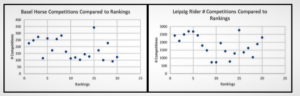
Linear regression can be a valuable tool to compare parts of data to each other to determine relationships. In this project, it was deemed, based on the complexity of multiple regression analysis, that two variable comparisons would be more appropriate for this data set. In two variable linear regression, the relationship between two numerical lists of data with the same number of elements is graphed often using technology. The graph assigns one variable to the x-axis and one variable to the y-axis. If the variables show a relation to each other, the graph will show a line of best fit roughly in between all of the data points. Preferably, a linear regression graph should have an “r” number, or a number that indicates the correlation/mathematical relationship strength, of r>0.7. The linear regression analysis of the data began with the creation of 50 Excel scatterplots examining five initial two variable relationships for each of the ten competitions (see Figure 2). These assisted in selecting variables for the creation of linear regression graphs. The Excel data was then used to create 100 linear regression graphs using StatKey to see if there were any strong correlations between different combinations of the following nine variables to determine which factors could be used for the creation of a mathematical model (an example of one of the regression graphs shown below in Figure 3). All of the graphs in the mathematical analysis were not included in the paper in the interest of brevity [7,13].
Horse Age
Horses in both the total competitors and top 20 for each event ranged from 8-17 years old, with the required age for competition being seven. The majority of these top 20 finishers were in the 10-14 age range. A theory that older horses may have more trouble in the competitions requiring 165 cm (65 inches) versus 160 cm (63 inches) maximum jumps was tested with regression but did not show a strong correlation proving this was the case [7].
Rider Age
Most riders competing had an average age of 34-40, with a range from 18-59 years old. There was a greater percentage of riders of ages 29-39 placing in the top 20 than the other age groups [7].
Horse Month of Birth
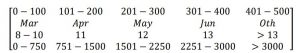
Horse month of birth was examined by assigning the values one through 12 for each month, in addition to creating comparison graphs for quarters of the year, where the twelve months were divided evenly into three-month segments assigned the numbers one through four. Show jumping horses keep their actual birth dates, unlike the assigned January 1st birth date for Thoroughbred race horses [9]. In the study of the ten 2019 competitions, horses were mostly born in the March-June range [7]. This is consistent with the natural horse breeding season. The season starts in mid-April and goes through early summer, with the gestation period of the horse being about 340 days. That results in horses being born about March to June [7,10-11]. Before this was found an interesting theory was postulated that it may be tied to such phenomena as seen in human hockey players, that many players have birth dates at the beginning of the year because their age and size when applying to enter the sport put them at a competitive advantage [12].
Horse Total FEI Competitions
The majority of horses in both the total and top 20 competitors had completed between 100-200 competitions. All top 20 horses had completed between 31-461 competitions. Horse jumping careers were limited to only hundreds of competitions, probably due to aging concerns leading to injuries or declining ability to jump at these heights [7].
Rider Total FEI Competitions
Most of the riders placing in the top 20 had completed between 1,000-3,000 competitions. Out of top 20 riders, the range was 446-3,779. This number may seem sizable at first, but it is important to note that each competition is a multiple day event (with the World Cup typically on the last day) of different riding contests that are each counted as part of a rider’s experience [7].
Horse/Rider Days Since Competing
Horse days and rider days since their last multiple-day competition were examined with regression analysis, but it was apparent many riders were riding similar events in the same season, so this did not seem to be a contributing factor. Also, when there was a gap, it was unknown if it was due to veterinary reasons, rider injury, or competitive reasons [7].
Rider Gender
Both horse and rider gender were examined in the regression by assigning the number one to males and the number two to females. In regards to rider gender, men and women do not compete in separate events. Men typically placed higher on average than women in all of the events. One potential reason for this may be that the average number of competitions of all the female and male riders was always higher for men, thus meaning they may be considered more experienced. Out of the 334 rider performances studied in 2019, 84 percent of the riders were male. Out of the top 20 rider performances over the ten competitions, 90 percent of these were male. This is notable when realizing that one of the reasons most of the top 20 competitors are men is that there is a high percentage of men competing overall when compared to women [7].
Horse gender
For the horse genders, out of the 334 horse performances studied in 2019, 71 percent of the horses were male (geldings and stallions were grouped together). Out of the top 20 horse performances over the ten competitions, 71 percent of these were male [7].
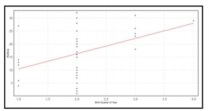
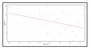
The correlations found among the 100 graphs made showed low correlation r-values ranging from -0.0059 to 0.433. The coefficient of determination, another measure of coefficient strength, is referred to as r2 and can have values ranging from zero to one, with one being all data points on the same curve with perfect correlation. The r2-values found ranged from 0.00003481 to 0.187489 [7,13]. These correlation findings indicate that a linear regression model is not appropriate for this particular data set. The highest correlation is shown in Figure 3 below, an r-value correlation of 0.433 between horse birth month by quarter of the year and ranking result for the 2019 Amsterdam competition. Viewing these results, a decision was made to pursue Linear Algebra to determine any correlations that could not be revealed with linear regression that could be used to build the model [7,13].
Linear Algebra Model
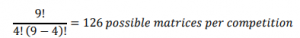
Linear Algebra is a field that incorporates matrices, or arrays of numbers that organize data and equations for mathematical analysis, to be able to examine, analyze, and model different data sets. It was determined that this discipline would contribute to this particular study because it could be used to correlate four different variables at once, and could be used to experiment with different assortments of variables to attempt to find the ideal combination for a model. Discovering the correct combination was very much an experimental process, given that there were nine variables examined with four categories that could be compared at one time, 126 different matrices could have been made for a total of 1,260 matrices across the ten competitions, as calculated in the below Equation 1. To narrow the matrices out of this group that would have to be created to make the analysis possible, it was necessary to further analyze the factors and their possible contributions.
Due to linear regression not revealing any major links between variables, it was necessary to look at the proportions of different factors among the top 20 and total competitors for each of the ten studied competitions. For instance, as previously mentioned, most riders in the top 20 had completed between 1,000-3,000 competitions. It was also illuminating to examine the counts of the total horses by birth month for all ten competitions, as that showed a very strong tendency for horses to be born in the spring, as explained above. Additional percentage comparisons aided in the selection of the initial four factors to include in the first set of matrix analysis: rider gender, horse birth month, horse age, and the rider’s career FEI competitions [7].
Initial Stage
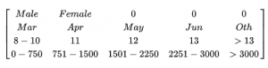
In the first stage of the linear algebra analysis, matrix multiplication was used as a way of measuring the spread of the data and seeing if the combination of the four factors chosen had a significant enough effect on rankings. A primary matrix was created for each competition that displayed the percentage of each category that was found in the top 20 riders for each competition, as shown in Matrix 1. The first row is the percentage of male vs. female riders, the second row is the percentage distribution of horse birth months, the third row is the distribution of horse age in years, and the fourth row is the rider’s career FEI competitions [7].
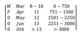
Then for each of the top 20 competitors in the studied ten competitions, a matrix was created that described the description of each horse and rider pair (200 total matrices). The rows and columns of the categories had to be reversed to make matrix multiplication possible, because a 4×5 matrix can be multiplied by a 5×4 matrix because the numbers in the center are the same (see Matrix 2). Because each matrix for individual competitors was being compared to overall competition proportions, instead of the individual matrices having percentages, they instead had a one or a zero to indicate if the horse and rider pair met that criteria [7].
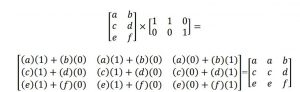
Each individual matrix of the top 20 was then multiplied separately by the main competition matrix for each of the ten competitions (200 total matrix multiplications). An example of the process of matrix multiplication is shown in Matrix 3. This resulted in a matrix result that showed the trace score for each horse and rider on the main diagonal for the resulting matrix (as shown in Matrix 4). A trace score is a measure of the spread of the data values over the categories in the resulting matrix [15]. It is found by adding the values of the diagonal in the matrix found. These trace scores were correlated to horse and rider pair rankings using StatKey, and no correlations were better than r=-0.332 (as shown in Figure 4) [7,13].
Creation of Predictive Model
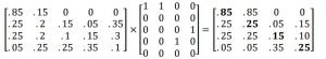
The again less-than-ideal correlation results showed the need to explore further linear algebra analysis. First the matrix for each competition needed to be adjusted because the weight, or proportion of the data that may have been too heavily influencing the results, was too heavy on rider gender, given the division at 0.85 and 0.15. The percentage of men that placed in the top 20 out of total men competing was similar to that same proportion for women, so its exclusion from the database seemed reasonable. Based on the previous analysis in previous steps of the research, it appeared horse number of competitions may also influence rankings and would be worth exploring (modified matrix shown in Matrix 5). When the matrices were adjusted, experience for both the horse and rider seemed to be significant [7].
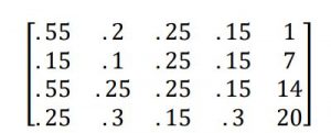
The above Matrix 5 was created for each of the ten competitions based on the proportions of the top 20 competitors in each. Then the matrices for the 1st, 7th, 14th, and 20th horse and rider team were multiplied by this new matrix for each competition and the trace scores were found, for a total of 40 matrix multiplications across the ten competitions. These numbers were selected for a somewhat even spread over the data. These trace scores were entered into equations with variables and set equal to the 1st, 7th, 14th, and 20th numbers (as shown in Equation 2). A linear algebra technique called finding a reduced echelon form (explained in Matrix 6) of a matrix was used to find the resulting coefficients (numerical multiples of variables that indicate their proportion) for these equations to use to create a model for each competition [7].
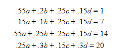
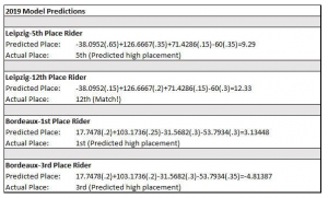
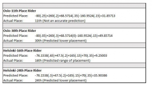
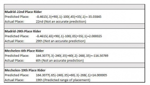
After solving the set of four equations, these numbers could be used to create a generic equation for each competition that could be used by looking at the features of a horse and rider pair at a certain ranking, entering these proportions into the model, and checking if the rider’s predicted placement matched the actual placement (Examples shown in Equations 3,4). These matrix operations produced an equation for six of the ten competitions. The attempt to create models for the other four competitions may require further adjustments to the matrix proportions or other factors may need to be included [7].


2018/2019 Comparison
Individual riders that competed in the same location in both 2018 and 2019 were compared using the model for that location to view if it predicted placement. After the testing of three riders it was determined that the values were varying so greatly a year-to-year comparison was not realistic. This was possibly due to the fact that competition proportions were originally used to create each model, so the model is not transferable to a competition that does not have similar proportions of horses and riders. Two riders were tested for each of the six competitions from 2019 that yielded a mathematical model to test if the model functioned if not using the 1st, 7th, 14th, or 20th rider (see Table 2 below). Of the twelve, only one test predicted a rider’s placement accurately. Of the others, in seven of the twelve tests, the model at least predicted if the rider would be in the top or lower place finishers [7].
Conclusion
The combination of two methods of mathematical analysis led to the development of a model that was able to at least approximate competition placement in more than half of the tests. Applying linear regression analysis to the data set led to the finding that no single factor was a main contributor to competition success and a set of factors needed to be explored. The application of Linear Algebra, (after linear regression did not provide enough information) resulted in the creation of models for six of the ten studied 2019 competitions. Each competition and location may have its own combination of unique factors resulting in certain performers doing well, which is likely why all six modeled competitions had different coefficients [7,13]. In total, during the research and analysis stage of this paper to select factors, create, and refine the model, 50 scatterplots, 100 linear regression graphs, and over 240 matrix multiplications were created and performed.
The limited success of these models was likely due to a variety of factors. The factors that could be studied numerically was limited, information on certain factors was unavailable, and sport participants may know information from being in the field such as who has the best trainers and riding instructors, etc. At this level of competition, it may also be that all of the horses and riders are so evenly matched in the easily quantifiable categories that using these to accurately predict placement is difficult [7]. Non-quantifiable factors that certainly also play a part are horse and rider grit and determination, which are difficult to correlate, as some things just cannot be measured.
Acknowledgements
In the Discrete Structures honors course the author took this past fall semester, the professor, Dr. Mike Long, was kind enough to encourage students in the class to submit a potential article for this research journal and made constructive suggestions towards ways to model this particular data set. Dr. Loretta FitzGerald Tokoly and Professor Kristel Ehrhardt provided excellent guidance and countless hours of their valuable time to assist in turning the author’s idea of looking at statistics from equestrian show jumping competitions into a mathematical model.
Contacts: agermain@howardcc.edu, a.germain@email.msmary.edu
References
[1] A. Stinner, “The Physics of Equestrian Show Jumping,” The Physics Teacher, vol. 52, pp. 202-206, Apr. 2014. Accessed Dec. 27, 2020. doi: 10.1119/1.4868930. [Online]. Available: https://pdfs.semanticscholar.org/baaa/4aa774d750320929cc5dd2f733ca0b17a6d9.pdf
[2] Neatorama. “Horse Calculus.” Neatorama.com. https://www.neatorama.com/2011/04/26/horse-calculus/ (accessed Dec. 27, 2020).
[3] J. Williams. “Performance Analysis in Equestrian Sport.” Comparative Exercise Physiology. https://www.wageningenacademic.com/doi/10.3920/CEP13003 (accessed Jan. 12, 2021).
[4] D. Marlin and J. Williams. “Faults in International Showjumping are Not Random.” Comparative Exercise Physiology. https://www.wageningenacademic.com/doi/abs/10.3920/CEP190069 (accessed Jan. 12, 2021).
[5] Evention TV. Walking Distances & Building a Safe Show Jump Course. (Jan. 30, 2013). Accessed: Dec. 26, 2020. [Online Video]. Available: https://www.youtube.com/watch?v=v_wCm0T-QMY
[6] Hamood, Paula. How to Train Straightness and Angles in Show Jumping with Paula Hamood, (Nov. 2, 2017). Accessed Dec. 27, 2020. [Online Video]. Available: https://www.youtube.com/watch?v=kewmPOZCKnM
[7] FEI. Competitions from 2018/2019. “FEI Database” [Online]. Available: https://data.fei.org/Calendar/Search.aspx
[8] Catapult Films, Laussane, Switzerland. Federation Equestre Internationale (International Equestrian Federation). (Dec. 20, 2013). Accessed: Dec. 26, 2020. [Online Video]. Available: https://www.youtube.com/watch?v=y4aNOsnpbw0
[9] J. Caldwell. “Why do Thoroughbreds Share the Same Birth Date of New Year’s Day?” Kentucky Derby. https://www.kentuckyderby.com/horses/news/why-do-thoroughbreds-share-the-same-birth-date-of-new-years-day (accessed Dec. 27, 2020).
[10] K. Anderson. “Mare Seasonality.” Cooperative Extension System. https://horses.extension.org/mare-seasonality/ (accessed Jan. 13, 2021).
[11] K. Anderson. “Management of the Pregnant Mare.” Cooperative Extension System. https://horses.extension.org/management-of-the-pregnant-mare/ (accessed Jan. 13, 2021).
[12] M. Gladwell, “The Matthew Effect,” in Outliers: The Story of Success, 1st ed. New York, NY: Hachette Book Group, 2011, ch. 1, pp. 15-34
[13] StatKey. “Descriptive Statistics for Two Quantitative Variables.” StatKey. https://www.lock5stat.com/StatKey/descriptive_2_quant/descriptive_2_quant.html (accessed Dec. 31, 2020).
[14] FEI. Helsinki, Finland. Re-Live/Jumping-Longines Grand Prix/Helsinki(FIN)/Longines FEI Jumping World Cup. (Oct. 20, 2018). Accessed Dec. 27, 2020. [Online Video]. Available: https://www.youtube.com/watch?v=ptJmiwzBNeM
[15] Lay, et al., “Chapter 7,” in Linear Algebra and Its Applications, 5th ed. [Online].
