
8 HCC’s Next Generation of Exoplanet Research
Nichole Warner, Howard Community College
Farah Alabdulrazzak, Howard Community College
Johnathan Hernandez, Howard Community College
Bryan Cheung, Howard Community College
Mentored by: Brendan Diamond, Ph.D.
Abstract
As the field of exoplanet research has progressed, further improvements to the quality of data are necessary to detect more subtle signals. Four aspects of the HCC telescope’s hardware were analyzed in our research: the impact of telescope rebalancing, uniformity of focus, choice of calibration method, and linearity of the camera. Rebalancing the telescope has significantly improved telescope tracking, as before rebalancing the drift was 6.8 pixels/hour horizontally, and 2.68 pixels/hour vertically, and after rebalancing the drift was less than 0.25 pixels/hour in both the horizontal and vertical axes. For the focus, there was a clear systematic difference that yielded a focus that was not uniform, with the manufacturer’s adapter maintaining a focus of ±0.3 pixels across the camera, while the 3D printed adapter had a focus of ±2 pixels, possible corrections are discussed. The twilight sky was determined to be slightly more precise than images of a calibration light panel, with the twilight sky white calibration images yielding an average coefficient of variation of 0.84%, while the light panel white calibration images had an average coefficient of variation of 1.17%, indicating less uniform pixels absorbing the incident light from the panel. Finally, the camera detector was determined to be linear in its response to incident light, within the nine regions analyzed (an average coefficient of determination of 0.9995), and precise for measurements of light in these regions for exposure times greater than 10 seconds and a brightness less than 60000 ADU.
Introduction
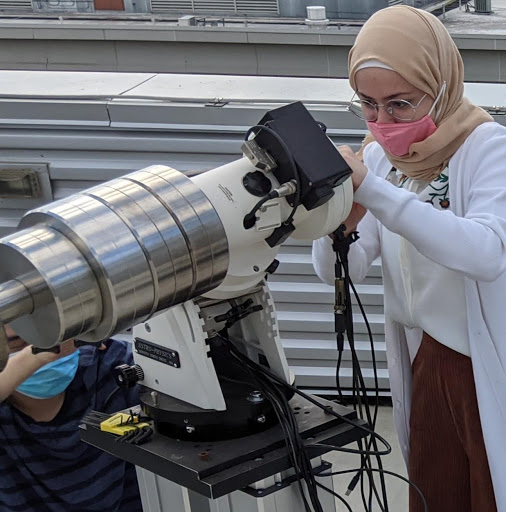
The exoplanet research group at Howard Community College has been conducting research on exoplanets for three years as a member of the Transiting Exoplanet Survey Satellite (TESS) Follow-up Observation Program (TFOP). The TESS detects the temporary drop in brightness in bright stars which may be caused by an exoplanet transiting across the disk of the host star [1]. The potential discoveries require further observations with ground-based telescopes. The main goal of the TFOP is to facilitate detection and measure masses of 50 exoplanets with a size less than 4 Earth-radii [2]. An important component of this work is to eliminate false positives or confirm detections [3]. The HCC exoplanet research team Hinchey, Jeffreys, and Samadani worked on assembling and operating the Planewave 0.36-meter telescope, Astrophysics 1100GTO mount, and SBIG 6303 Charged-Coupled Device (CCD) camera [4]. Deljookorani, Kunzle, and Leger built upon previous work, joined TESS, and submitted observations of possible exoplanets [3]. As TESS has progressed to its second phase of research, and observation targets are becoming increasingly subtle to detect and analyze with the necessary precision, this group focused on improving the performance of our hardware to allow for future research groups to keep up with the progressing TESS mission. Four significant factors were analyzed that may contribute to the precision of data collection: impact of telescope balance (Figure 1), uniformity of focus, choice of calibration method, and linearity of the camera. The results obtained by this research have elevated the level of understanding and operation of the Planewave 0.36-meter telescope, as well as the ability to utilize the telescope more effectively for future TFOP submissions.
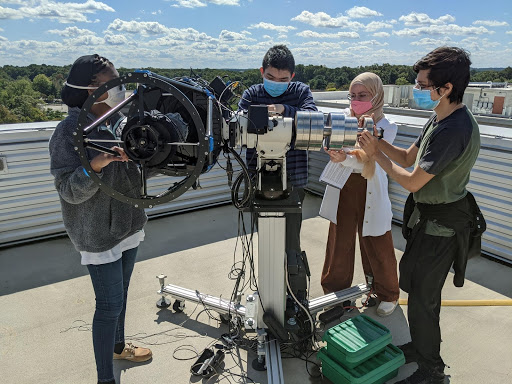
Telescope Rebalancing
The first objective was to determine if the telescope’s precision of tracking target stars was able to be optimized through rebalancing. The initial balancing, which was when the telescope was first assembled, was completed without the camera mounted. Fine adjustments on telescope balance on the two rotational axes, cable management improvements, and a computer-aided polar realignment were performed on October 2nd, 2020. Exoplanet observation requires multiple hours of imaging the same star in the sky during the course of a night. An observation was made before and after the rebalancing to determine the change in drift on a target star, where a target drift of 0 indicates that the telescope is tracking precisely on the target star. Using the position data (FITS X and FITS Y) from the observations before and after rebalancing, best line fit equations were plotted along with the data to indicate the approximate change in the telescope drift over time (Figure 3).
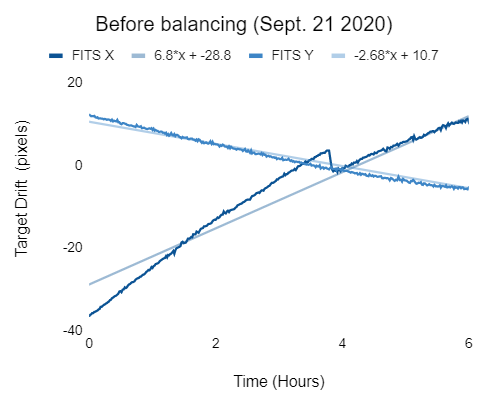
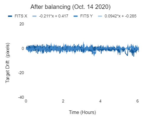
Through these equations, observations made before on the left of Figure 3 had a horizontal and vertical drift of 6.8 and 2.68 pixels/hour respectively while those made after rebalancing on the right of Figure 3 had drifts of less than 0.25 pixels/hour for both sides (with only small fluctuating drifts from the atmosphere being corrected during observations), indicating that the precision of the telescope has significantly improved. Since the CCD size is 3072 × 2048 pixels, the initial drift was still less than 3% of the overall image but would shift the star location by more than the Full Width Half Maximum (FWHM) of a typical star during an observation. The FWHM is used to describe the width of a Gaussian distribution, in this case the width of the stars (in pixels), to determine if there was a shift in the distribution of focus throughout the entire image. Improving the telescope tracking is achieved through precision balancing to minimize the load on the telescope mount motors. If a target star can be imaged on the same pixels of the camera for an entire observation session, this reduces the impact of systematic uncertainties from other sources such as different calibration of pixels and uniformity of focus across the camera.
Uniformity of Focus
The main purpose of this experiment was to see if there is a direct correlation between using different adapters and the effect on the overall focus of the telescope. To reduce the nightly telescope setup time, a group of students in the Engineering Department at HCC developed and designed a 3D printed quick clip adapter to replace the manufacturer’s adapter that required four bolts to be installed every night the telescope was used. This adapter was changed in fall of 2019 but until this paper there had not been any study of the impact on the telescope’s focus. Images taken before and after the installation of the 3D printed adapter were analyzed. The two images contain a dense field of stars, and both images were broken up into nine equal regions and within each region ten stars were selected, as well as other information about the set of bright stars in each region was recorded: position X, position Y, brightness, and Full Width Half Maximum (FWHM). The position X and position Y are the pixel positions of the selected stars in the X and Y axis, respectively. Once all the data from the stars amongst the nine regions were collected, then the set of data was analyzed to see if there were any trends amongst each row of regions (left to right) throughout the image. These calculations were performed for both images to try to see if there were any noticeable trends. After that, two graphs were plotted for both images, one being a FWHM vs Position Y graph and the other a FWHM vs Position X graph to look for trends in the data.
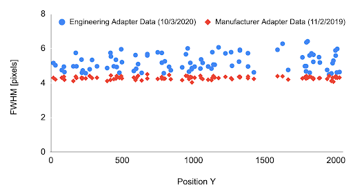
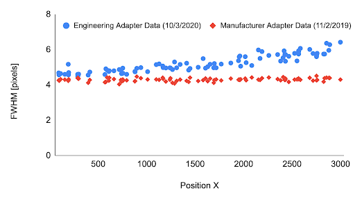
In Figure 4, the data is relatively flat indicating a uniform focus throughout the image, but for the 3D printed adapter (blue circles), the data is more scattered, which indicates a lack of precision in comparison to the data from the manufacturer’s adapter (red diamonds). In Figure 5, moving from left to right across the image, it is apparent that the 3D printed adapter (blue circles) has a positive slope, indicating a systematic shift in the focus, while the data in red remains flat. It was concluded that the manufacturer’s adapter maintained a uniform focus (±0.3 pixels) across the camera compared to the 3D printed adapter (±2 pixels). This is likely due to a slightly loose fit where the 3D printed adapter meets the telescope. The weight of the camera tilts the plane of the camera at an angle with respect to the plane of focus. Possible solutions include using the manufacturer’s adapter instead to maintain a uniform focus, or potentially modify and improve the existing 3D adapter designed by the Engineering Department students.
Choice of Calibration Method
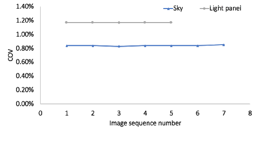
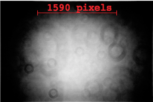
The CCD is utilized for capturing four types of images for each observation session: bias, darks, science, and white calibration images (Figure 7) [5]. White calibration images with high uniformity can be used to calibrate for the effect of dust that causes diffraction leading to systematic errors in the measured brightness [5]. These images can be obtained through images of the twilight sky, a white screen on a telescope dome, or an electroluminescent panel (light panel). The telescope used at HCC does not have a dome, it is covered with a fabric when not in use, resulting in the options of using the light panel or twilight sky. In this experiment, the pixels were tested to determine how much incident light is absorbed when using sky twilight versus an Aurora brand light panel [6], and how much the brightness changes across a specific region of the image was calculated in both methods. The two methods were compared to see which one generates images with a lower coefficient of variation across the pixels as shown in Figure 6. The uniformity in brightness across the pixels in the images were compared using Standard Deviation (SD), Coefficient of Variation (COV), and the average for COV as the comparison involved images with different mean values for the brightness. The COV is defined:
COV (%)= (SD/Mean) * 100
A higher average COV percentage indicates less uniformity of pixels receiving incident light, requiring a stronger calibration correction, which may lead to less precise images. The average COV for sequence of images taken using skylight was 0.84%, and 1.17% for light panel images (Figure 6). Future exoplanet research groups may rely on sky images for having less average COV, making these images more precise over the light panel images.
The method used to obtain the data consisted of taking a sequence of 7 calibration images using sky twilight with exposure time ranging between 3 to 7 seconds. Then, an additional 5 images were taken using the light panel with an exposure time of 34 seconds for each image. The exposure times were specific to gain an average brightness, also referred to as an analog-to-digital units (ADU) count, of 25000 for all 12 images. Using AstroImageJ [7], standard deviation and median of the pixels in each image was obtained and transferred these data to Microsoft Excel to calculate the coefficient of variation across the pixels of each image. Lastly, the images from two methods were compared after plotting the data in a scatter plot graph (Figure 6).
Linearity of the CCD
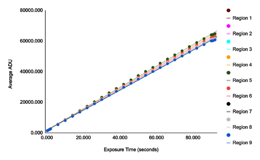
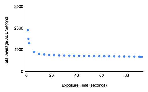
The CCD was also utilized to evaluate its linearity in response to incident light. CCD linearity analyzes the relationship between the brightness of the resulting image (measured in ADU), and how long the camera was exposed to light, and a linear response to light indicates that the pixels in the resulting image have a brightness proportional to incident light. If the two variables are correlated, there will be a linear shape when graphed, and the coefficient of determination, R2, will be close to one [8]. Similar methods used by Pereyra et al. were followed, in addition to evaluating the linearity of nine individual regions instead of the entire region of the CCD [8]. A series of five calibration images were taken at thirty-one different exposure times (between 0 and 92 seconds), using an Aurora brand light panel to span the full range of the detector (64000 ADU) [6]. The linearity was graphed for nine equal regions using the average ADU of the five-image series at each exposure time (Figure 8). The nine regions were numbered from bottom to top and left to right for the CCD image (1, 2, 3), (4, 5, 6), (7, 8, 9). The linear fits of the nine regions of the graph were distributed, due to the vignette effect, causing the center region to have the most light and highest ADU, regions surrounding the center region to have less light, and the regions in the corners to have the least light; there is also likely systematic error from the 3D printed adapter previously discussed in this paper (Figure 8). The linearity, determined by the coefficient of determination of each region in the graph, is an average of 0.9995 for the nine regions, using Microsoft Excel (Figure 8). This led to the conclusion that the CCD detector is linear in its response to incident light, and the detector is precise for measurements of linearity within the regions used for exposure times greater than 10 seconds and below 60000 ADU. With further analysis, a graph of the total average ADU per second compared to the exposure time revealed that there was an uncontrolled variable in the experiment, as the ADU/second vs. exposure time graph is expected to be nonlinear on the ends, and flat in the middle (Figure 9). The middle of the graph has a small negative slope, possibly due to a temperature drop from how long the telescope and CCD were outside (over three hours in October 2020; Figure 9).
Conclusion
The Transiting Exoplanet Survey Satellite that was launched by NASA four years ago has progressed to its second phase of exoplanet detection, which necessitates the contributing ground-based observatories to have higher precision observations to contribute to the extended missions. As the latest generation of exoplanet researchers at HCC, further improvements to the hardware were made along with methods to ensure high quality data is submitted to TFOP in the future. The rebalancing is expected to have the most significant impact to future data, though the quantification of the impact was beyond the scope of this paper and could be an area of future research. The improvement of tracking due to the precise balance will facilitate more comparison stars to be used in exoplanet analysis, since the field of stars will not shift significantly during the observation. It was also found that the focus has a clear systematic difference along the vertical axis of the CCD, likely due to a tilt when using a custom 3D printed adapter. There are two solutions; revert back towards using the original manufacturer’s adapter, or design an improved version of the adapter which would eliminate the tilt discussed previously. For the choice of calibration method, due to the smaller value of percent coefficient of variation within the pixels of twilight sky images, these images were concluded to be more precise over the images from the light panel. For future observation, obtaining calibration images through twilight sky will be preferred. Since both calibration methods have less than 1.5% variation the Aurora light panel may be a sufficient substitute when weather precludes twilight calibration images. The CCD was found to be linear in its response to incident light, with an average coefficient of determination of 0.9995 for the nine regions, and is precise for measurements of light in these regions for exposure times greater than 10 seconds and not exceeding 60000 ADU. These factors will provide future exoplanet research groups with a guide to operating the telescope more precisely than ever in the history of the HCC exoplanet research program.
Acknowledgments
NSF – This material is based upon work supported by the National Science Foundation under Grant No. 1458149.
The authors wish to thank the Engineering students who designed and built the 3D printed adapter for the telescope, Sean Koo, Brandon Tringa, Roberto Wilkerson, and Muhammad Anwar UI Haq installed on November 12, 2019. This greatly sped up the opening and closing of the HCC observatory.
Contacts: nichole.warner@howardcc.edu, farah.alabdulrazzak@howardcc.edu, johnathan.hernandez@howardcc.edu, bryan.cheung@howardcc.edu, bdiamond@howardcc.edu
References
[1] G. R. Ricker and et al., “Transiting Exoplanet Survey Satellite (TESS),” Journal of Astronomical Telescopes, Instrument, and Systems, vol. 1, no. 2015, 2015.
[2] “TFOP Overview,” MIT, [Online]. Available: https://tess.mit.edu/followup/. [Accessed 26 Feb 2021].
[3] S. Deljookorani, V. Kunzle, and D. Leger, “Exoplanet Photometry and False Positives,” Journal of Research in Progress, vol. 3, 2020.
[4] J. Hinchey, W. Jeffreys and P. Samadani, “Fantastic Exoplanets and Where to Find Them,” Journal of Research in Progress, vol. 2, 2019.
[5] D. M. Conti, October 2018. [Online]. Available: https://www.astrodennis.com/Guide.pdf. [Accessed 8 February 2021].
[6] “Aurora Flatfield Panels,” Gerd Neumann, [Online]. Available: https://www.gerdneumann.net/english/astrofotografie-parts-astrophotography/aurora-flatfield-panels/uebersicht-aurora-flatfield-panels-overview.html. [Accessed 26 Feb 2021].
[7] Cornell University, “AstroImageJ: Image Processing and Photometric Extraction for Ultra-Precise Astronomical Light Curves (Expanded Edition),” [Online]. Available: https://arxiv.org/abs/1701.04817. [Accessed 2021].
[8] A. Pereyra, M. I. Zevallos, J. Ricra and J. C. Tello, “Characterizing a CCD detector for astronomical purposes: OAUNI Project,” Revista TECNIA, vol. 26, no. 2, pp. 20-25, 2016.
