
Exoplanet Photometry and False Positives
Shila Deljookorani, Howard Community College
Veronica Kunzle, Howard Community College
Dominic Leger, Howard Community College
Mentored by: Brendan Diamond, Ph.D.
Abstract
The goal of our research is to assist in the confirmation of exoplanets, which are planets outside our solar system. This is accomplished through participation in the Transiting Exoplanet Survey Satellite (TESS) Follow-up Observation Program. The satellite detects a temporary drop in brightness in a star which then requires further observations with ground-based telescopes. One of our primary objectives with the TESS collaboration is to identify false positives, primarily due to eclipsing binary stars where two stars are orbiting one another in close proximity. Over a single night, a few hundred images are taken using a 0.36m telescope at Howard Community College. The time series of images can corroborate any dip in the brightness of the target star or seek alternative sources for the initial signal. We will present examples of false positives detected with our telescope, and how to differentiate between a transiting exoplanet and an eclipsing binary star system.
Introduction
Exoplanet transit photometry, also known as the transit method, is the measurement of a drop-in brightness of a star over a period of time, due to an orbiting planet around the star. Any planet outside of our solar system is called an exoplanet. Each time an exoplanet passes in front of its host star (transits), the planet blocks a small fraction of the star’s light. The graph of brightness as a function of time is created from a series of images. This graph is known as a light curve. A false positive is any event that can mimic an exoplanet transit. Our research group at Howard Community College is part of an international collaboration of scientists working to identify false positives from new exoplanet discoveries. We joined the TESS Follow-Up Observation Program (TFOP) in July of 2019. As a member of TFOP, we assist with observational evidence to indicate if the Transiting Exoplanet Survey Satellite (TESS) has detected an exoplanet candidate or a false positive. By using smaller research telescopes such as at HCC with high magnification, the TFOP is able to obtain higher resolution images then the wide-angle all-sky survey camera on board TESS. This also prevents waste of valuable large telescope time on follow-up observations by large telescopes such as the James Webb Space Telescope (JWST) if false positives are removed from planet candidate databases [1].
False Positives
A drop in a star’s brightness is not primarily due to a transiting exoplanet; the drop could be an indication of another object passing in front of the star also known as a false positive. Identification of false positives are made primarily through the shape of a light curve, alternating shape, percent depth, or using different colored filters.
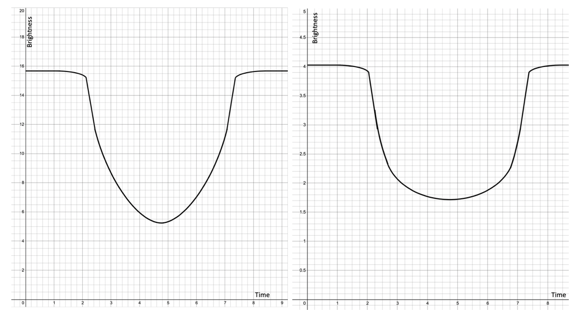
One primary indicator that distinguishes an observation as an exoplanet or a false positive is the shape of the light curve. The different shapes are produced due to the varying sizes of the objects passing in front of the star. Figure 1 below compares the differences between a v-shape light curve and exoplanet light curve. The v-shape light curve (left) would have a larger drop in brightness; and is commonly due to an eclipsing binary star system (EB). An eclipsing binary system is a two-star system that orbits each other; as they orbit when the smaller star passes in front of the bigger star, it produces a more significant drop in brightness. Although both stars are emitting light, the transiting star, relative to the observer, is still blocking out a portion of the light from the other. The exoplanet light curve (right), has a much smaller drop in brightness, this is due to the transiting object being much smaller than its host star, thus blocking out a much smaller fraction of light. The exoplanet graph will also have a faster decline in light, with an essentially constant base, then finally increase once again, thus creating a bucket-shaped curve.
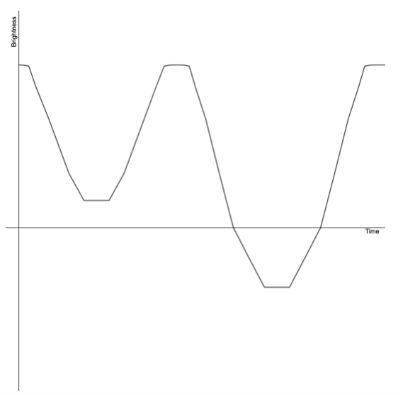
The alternating v-shaped false positives are due to multiple transits occurring on the observed star. Figure 2 below is a representation of how a v-shape alternating light curve would appear. The primary causation of these dips are also caused by eclipsing binaries (EB); these star systems are orbiting around a center of mass. When both a dimmer star and a brighter star are in the field of view, their emitting light combines creating a constant light graph. However, due to the position of the observer, we see the star system orbiting each other. As these stars orbit around each other, they produce a variation in a drop brightness. As the dimmer star passes in front of the brighter star (secondary eclipse), we have a smaller drop in brightness. As the dimmer star occults (passes behind), the larger star (primary eclipse), it will result in a more significant drop in the brightness. Looking at Figure 3 below, the first decline in brightness is representing the secondary eclipse, and the second drop is representing the primary eclipse.
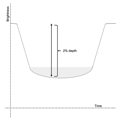
Another factor we look for when differentiating between an exoplanet transit and a false positive, is the percent drop in brightness. As mentioned previously, an exoplanet light curve would have a much smaller dip in brightness compared to a false positive. As we observe and produce a light curve graph, our data will tell us the percent drop during the transit. Planets are smaller than stars, and there is a maximum dip in the brightness that would indicate that we are looking at a false positive. When we have a transit that has over a 2% drop in brightness, we can predict that the observation is a false positive, rather than an exoplanet transit. The 2% dip is far too large for the causation to be an exoplanet. In Figure 3 below is a representation of the dip in brightness we could observe.
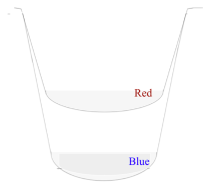
Obtaining images with different filters help us to distinguish an exoplanet transit from an eclipsing binary system; since different stars give off distinct colors due to their temperature and sizes their depths will be different once data is processed to create a light curve. Depth variations in when using various filters gives an indication of a possible EB. This is another reliable indicator for another type of false positive. In Figure 4 below, there is a light curve represented in two different filters. The red filter has a much shorter depth than the blue filter, indicating that there are two different stars being observed. If the event had been caused by the silhouette of an exoplanet, the drop-in brightness would be a consistent depth across all photometric filters.
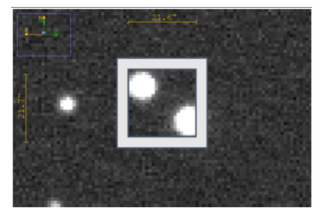
The TFOP program concerns follow-up observations with the data given to us by TESS. TESS uses larger pixels since it has such a wide field imaging range; thus, it is unable to differentiate between different light coming from different stars. Figure 5 shows how one TESS pixel (21 arc-seconds) is significantly larger compared to our pixels (0.72 arc-seconds). Ground-based telescopes have a much higher resolution; we can distinguish between the light coming from different stars. Without the blending of light and the higher resolution, we also assist in producing evidence of whether a transit is an exoplanet or false positive.
Materials and Methods
Our primary observation setup consists of a Planewave 0.36-meter telescope, SBIG 6303 CCD (camera), and a computer in a control room that runs the observation software. We use a confidential database of potential planet candidates from the TFOP to select our targets for our observations based on position, brightness, depth of transit and other factors. The main observation software consists of the programs MaximDL and Maxpoint, used for telescope controls and image tracking. In order to process data, we use AstroImageJ, an image processing program designed explicitly for exoplanet photometry [2]. The hardware setup is the same as the previous exoplanet research team featured in JRIP 2019 [3]. Previous observations following a similar set of methods can be seen in the Astronomical Journal article below [4].
MaximDL software allows us to control the telescope and move it into the target position to start capturing images. One of the main functions of this program is to resolve the position of the telescope, to allow precision tracking using a secondary guiding camera. Maxpoint is software that further improves tracking as well as the pointing of the telescope. Maxpoint models the telescope’s gears in the mount based on 50 to 100 stars evenly distributed across the full sky from a calibration night [5]. To limit systematic errors in the response of different parts of the CCD, tracking is maintained on a target star within a couple arcseconds of angle, corresponding to only a couple of pixels position.
In order to collect accurate data, there are parameters of the chosen target start given to us from TFOP that we need to take into consideration. These parameters involve the duration of the transit, the magnitude of the star, and the projected depth of the light curve. These variables control how we set up our telescope, as well as how long we would be taking images. MaximDL needs to be configured one more time to automatically take images and save them to a specific file location. We use a feature from MaximDL termed autosave, which allows the automatic taking of images to be saved to a specific file. Once autosaving is set up, the next thing to do is make sure tracking is maintained, and image saving is working throughout the observation period. The image taking process must begin prior and end later than the actual transit time in order to ensure there is a baseline of data.
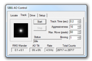
A useful component of our imaging system is the tip/tilt autoguiding, also known as adaptive optics. This is a hardware upgrade to the SBIG CCD that is controlled through MaximDL in order to compensate for vibrations in the telescope and atmospheric turbulence. Autoguiding is done by rapidly moving a thick window in front of the CCD to offset the image, allowing for precise images to be taken even when the target star is moving [6]. Figure 6 shows the tracking menu of the SBIG AO controls, which allows for several options to be modified in order to accommodate varying observation conditions. Tracking and adaptive optics increase the precision in our observations and allow us to take better images and look at more difficult targets with greater confidence.
In order to process our data, we use AstroImageJ, which is a derivative of the program ImageJ that is explicitly designed to be used with exoplanet photometry. Prior to processing our images, we first sort them and remove images with poor quality. This low quality can be caused by a variety of factors, such as a temporary loss of tracking, a power loss to one or more components, or an object getting in the way. Some images may also be taken without specific FITS header (image metadata) components, which requires them to be processed again through AstroImageJ to add necessary FITS header information. Once all the poor-quality images are removed from the rest of the image stack, the images can be appropriately calibrated as described by the exoplanet research team featured in JRIP 2019 [3].
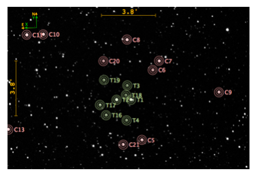
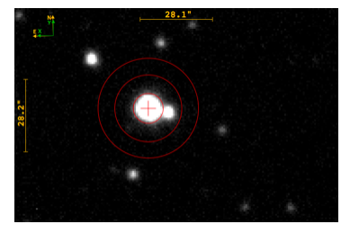
While the private TFOP database gives us coordinates for a predicted transit event occurred according to TESS’s data, it does not guarantee there is a transit event on the listed star. In order to locate the event, we need to select several target stars and comparison stars. These target and comparison stars should all be of similar brightness and size, but they can vary slightly between each star if needed, as seen in Figure 7. Once our target and comparison stars are selected, we use AstroImageJ to automatically repeat the star selection for all the other images within the calibrated image stack, and we can then resolve a graph from it. AstroImageJ compares the comparison and target stars using an aperture and annulus to measure the brightness, as shown in Figure 8. Additional information regarding this process can be found in an article published by Cornell University [2]. The graphs developed from this process still need to be adjusted in order to match TFOP standards. These standards ensure a high degree of clarity in each graph, and all submissions to the TFOP database must be raised to them prior to submission. Once those options are modified, and the graphs are raised to TFOP standards, the image processing is completed, and a report can be sent to the collaboration. For a more detailed analysis on the methods to find false positives, see the article by Dennis Conti below [7].
Results
Throughout our time participating in the TFOP program, we have contributed ten successful observations to the TFOP database of exoplanets maintained by MIT [8]. Our observations are limited to a minimum depth of 4 parts per thousand (ppt), meaning that objects that block very little light of their host star cannot be observed effectively using our equipment.
Of the ten observations listed below in Table 1, seven were labeled as false positives. These results are categorized as NEB, PC, BEB, and EB. Ingress refers to the spot at which the whole planet enters the star’s disc (start of the transit), and Egress refers to the point at which the planet reaches the opposite side of the star’s disc and exits from it (end of the transit) [9].
| Target | Obs. Date | Depth (ppt) | Result | Observation Summary |
| Jul. 27, 2019 | 35 | EB |
Known EB used to verify our data reduction procedures. Full transit. |
|
| Jul. 30, 2019 | 300 | NEB |
Known EB used to verify our data reduction procedures. Full transit. |
|
| Aug. 11, 2019 | 20 | BEB | Full transit. Combined observations showed chromaticity. | |
| Sept. 26, 2019 | 80 | NEB | Ingress +70%. | |
| Oct. 23, 2019 | 8 | PC |
Full transit. Possible large planet (9 REarth) |
|
| Oct. 24, 2019 | 10 | EB | Ingress +20%. Later observations showed V-shape curve. | |
| Nov. 02, 2019 | 80 | NEB | Full Transit. | |
| Nov. 07, 2019 | 8 | PC |
Egress +40%. Possible large planet (16 REarth) |
|
| Dec. 22, 2019 | 10 | BEB | Full transit. Confirmed BEB with TFOP spectroscopic observation. | |
| Dec. 24, 2019 | 3-6 | PC | Full transit in g’ and r’ filters. Depth is near our equipment uncertainty so requires high precision follow up observations. |
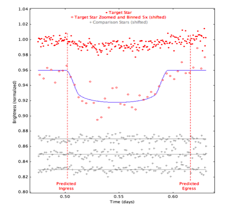
Figure 9 is an additional graph for our observation on October 23rd, 2019. After analysis in AstroImageJ, we found that the graph showed signs of being an exoplanet candidate. The drop-in brightness of the target star was calculated at 0.08%. In order to ensure that this was not caused by an eclipsing binary and was a possible exoplanet transit, follow up observations were conducted by other groups using different light filters to look for chromaticity such as in Figure 4. The follow up observations showed no change in the brightness drop, leading to the target star being labeled as a planet candidate in Table 1.
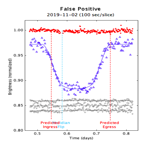
As shown above in Figure 10, the target star (in red) did not have a brightness drop, but the nearby star, TIC468845640-0 (in blue), unexpectedly did. The star dimmed as expected of an eclipsing binary throughout observation, with a deep V curve and rounding towards the bottom. As the target star and nearby eclipsing binary were orbiting each other, a portion of nearby eclipsing binary’s brightness was blocked due to their transit, mimicking a light curve of an exoplanet. This drop was measured using a Sloan r’ light filter and AstroImageJ calculated the peak depth of the drop at 7.92%. Once this high drop was found, the target was ruled as a false positive caused by an NEB.
Challenges
Our time spent working with the TFOP collaboration has yielded a lot of useful observations, however these only came after overcoming many challenging and unsuccessful experiences. We began to use remote observation and tracking this year, which were big steps to take for our group. While advancing into new territory between this year and last year has brought new progress, it also brought new issues unique to our project that we have learned from. For every observation we submitted to the exoplanet database, we had to terminate at least one other observation due to either bad weather, hardware issues, or software issues.
Poor weather conditions were a major limiting factor in our observations. There were many instances where the observation had been canceled before we had begun the observation process, due to a sudden overcast of clouds. Another weather factor that hindered our research was wind. Winds that we would experience every so often, would overwhelm the adaptive optics, ruining the images by causing the telescope to shake during image capture.
Hardware issues were also a limiting factor in our observations. While our availability was greatly increased by using remote observation, so was the potential for problems we could not solve without being on site. One of these issues was internet disconnection, causing the telescope to sit idle after finishing a meridian flip. Meridian flips are required in order to continue tracking on a target that is moving around our telescope, since the mount does not rotate completely. While this reorientation does normally cause us to lose one image, we couldn’t remotely restart tracking on the telescope, resulting in most of the observation being lost. Another issue that caused premature termination of observations was intermittent battery failures on the camera. While it was an effective method to protect the camera from a power surge, the battery failing ended up causing multiple observations to fail due to the inability to track or image with the CCD.
Software issues, while the rarest, were the most severe. In one of the two cases, the telescope was calibrated to the wrong orientation, which caused a failure in tracking. This ended up causing the telescope to rotate into the base of the pier. If it were not for the telescope automatically stopping, this would have caused serious damage to the telescope’s motors. Another problem was not noticed until after data processing. During the calibration phase, the camera’s shutter was open while taking some images where it needed to be closed. This created improper calibration images, which limited the quality of the final light curve.
Conclusion
Throughout the duration of our research project, our group has learned how to distinguish between a false positive and exoplanet candidate using exoplanet photometry. We used the telescope, CCD, and other equipment to observe target stars gathered from the TFOP database, and currently we have contributed 10 successful observations to the program. Through these, our group has been able to observe the major aspects of eclipsing binary false positive stars, including the large brightness drop, v-shaped graph, and chromaticity of the target star. Our November 2nd, 2019 observation in Figure 10 above is an example of all three characteristics, with the characteristic v-shape being the most prevalent of the three. Alongside that, the measured brightness drop of 7.92% added more evidence of this target being a false positive. Further follow-up observation showed chromaticity as well. The results of analyzing these false positive observations demonstrate that there is a difference between them and a normal exoplanet. Exoplanet brightness drops lack any chromaticity and do not have the characteristic v-shaped brightness drop seen in all false-positive binary stars.
Acknowledgements
This material is based upon work partially supported by the National Science Foundation under Grant No. 1458149.
Contacts: shila.deljoo@yahoo.com, verkun6430@gmail.com, dominicleger98@gmail.com, bdiamond@howardcc.edu
References
[1] G. R. Ricker and et al., “Transiting Exoplanet Survey Satellite (TESS),” Journal of Astronomical Telescopes, Instrument, and Systems, vol. 1, no. 2015, 2015.
[2] K. A. Collins, J. F. Kielkopf, K. G. Stassun and F. V. Hessman, “AstroImageJ: Image Processing and Photometric Extraction for Ultra-Precise Astronomical Light Curves (Expanded Edition),” Cornell University, Louisville, Kentucky, 2017.
[3] J. Hinchey, W. Jeffreys and P. Samadani, “Fantastic Exoplanets and Where to Find Them,” Journal of Research in Progress, vol. 2, pp. 2-11, 2019.
[4] K. A. Collins and et al, “The KELT Follow-up Network and Transit False-positive Catalog: Pre-vetted False Positives for TESS,” The Astronomical Journal, vol. 156, no. 5, p. 234, 2018.
[5] Diffraction Limited, “Maxpoint,” Diffraction Limited, [Online]. Available: https://diffractionlimited.com/product/maxpoint/. [Accessed 2020].
[6] Diffraction Limited, “SBIG AO Control,” Diffraction Limited, [Online]. Available: https://diffractionlimited.com/help/maximdl/MaxIm-DL.htm#SBIG_AO_7.htm. [Accessed 2020].
[7] D. M. Conti, “Exoplanet False Positive Detection with Sub-meter Telescopes,” Annapolis, MD, 2018.
[8] S. Seager, N. Guerrero, D. Latham and C. Burke, “TESS Observations,” Massachusetts Institute of Technology, 2018. [Online]. Available: https://tess.mit.edu/observations/. [Accessed 2019].
[9] D. M. Conti, “A Practical Guide to Exoplanet Observing,” 2018. [Online]. Available: https://astrodennis.com/Guide.pdf. [Accessed 2019].
