
Looking Closely: The Transit of Mercury
Grant Bunyard, Howard Community College
Mentored by: Brendan Diamond, Ph.D.
Abstract
On November 11, 2019, the transit of Mercury across the sun was observed through a Celestron C11 SCT and captured with a Nikon D300. Approximately 80% of the transit and the egress was captured. The research goal was to investigate what we could determine about the solar system from the data gathered during this transit. The diameter of Mercury was calculated within 1% using the data and known distances to Mercury and the Sun. Other applications included calculating the angular separation of Mercury and the Sun, calculating the angle of Mercury’s orbit, and analyzing a historical calculation of the distance from Earth to the Sun using Kepler’s Laws, first done in 1769. Other optical phenomena including the light curve, the black drop effect, and limb darkening were observed.
Introduction
Mercury is the closest planet to our sun, and the smallest planet in our solar system; it is only slightly larger than Earth’s Moon. About 13 or 14 times every century, Mercury’s orbit takes it in between the Earth and the Sun [2]. This transit can be observed from Earth. On November 11, 2019, Mercury transited across the sun for the first time in over 3 years, and for the last time in over 13 years [3]. Many conclusions about our solar system can be drawn from the transit. Throughout the day of November 11, 2019, a small team on the observatory of Howard Community College captured over 70 gigabytes of data in the form of pictures and videos of the transit. The data was analyzed mathematically and analyzed using multiple software programs. During this analysis of the images taken of Mercury, the diameter of Mercury was calculated, the angular separation of Mercury and the Sun was calculated, and the inclination of Mercury’s orbit was calculated. A historical calculation of the distance from Earth to the Sun that was first theorized by Johannes Kepler and Edmond Halley was repeated. The brightness of the Sun as a function of time during the transit, referred to as a light curve, was also analyzed. In addition, the optical phenomena of limb darkening, and the black drop effect were observed.
Diameter of Mercury
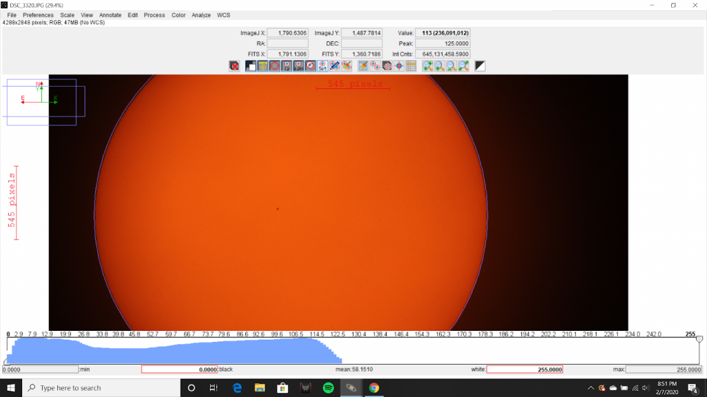
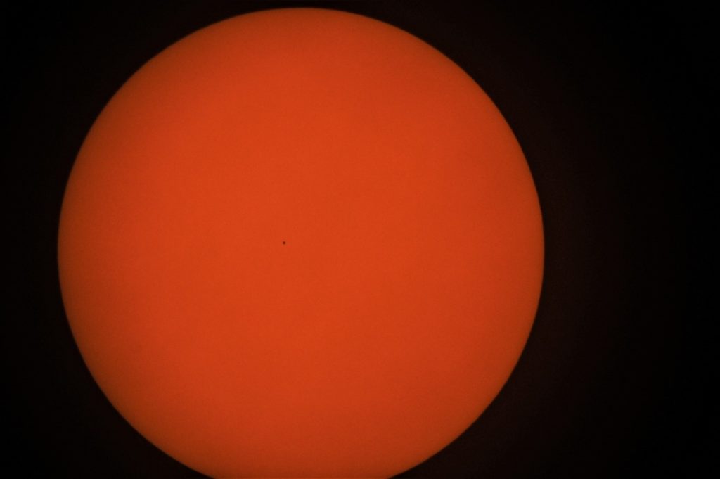
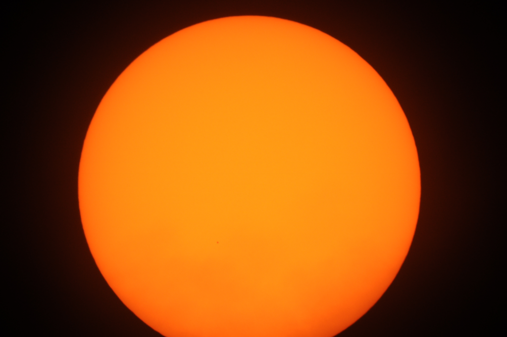
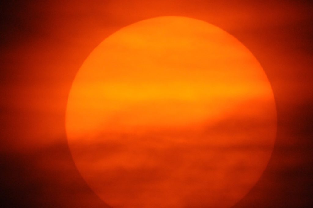
All measurements taken for calculations used in finding the diameter of Mercury were taken from image DSC_3320. This image was captured with a Nikon D300 camera through a Celestron C11 SCT telescope using a Helios Solar Glass filter. The filter used blocks over 99.999% of all incoming light and causes the Sun to appear orange rather than white [4].
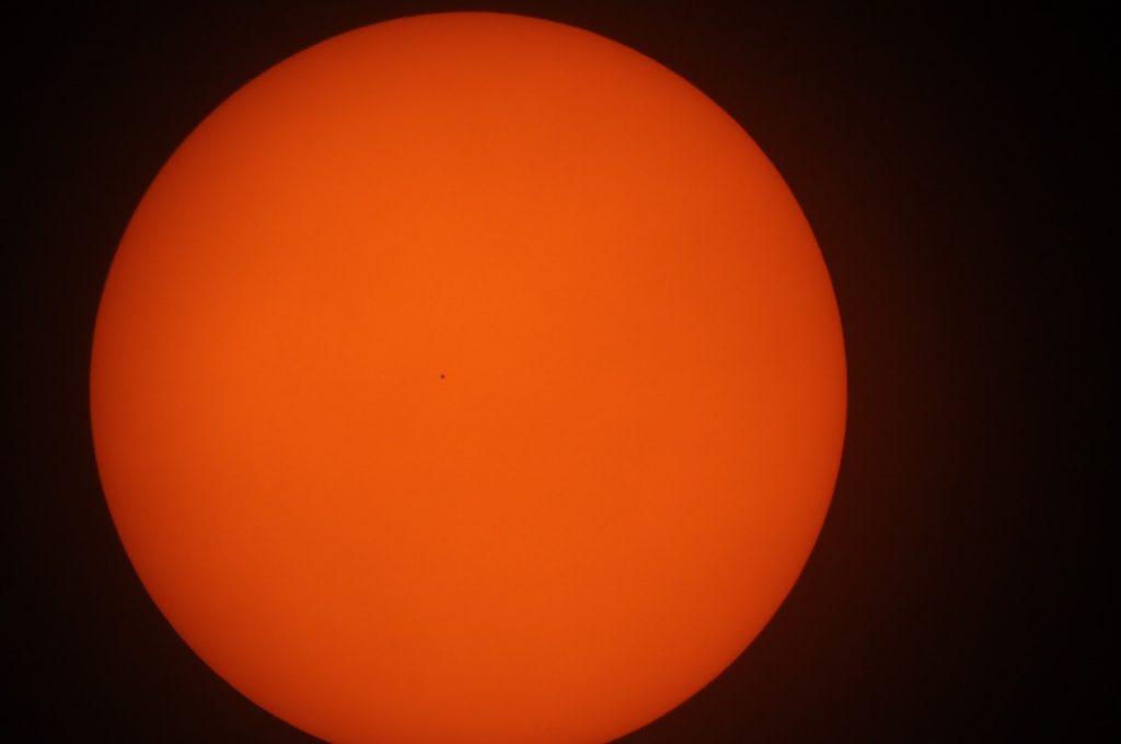
The relative size of Mercury compared to the Sun’s image was calculated from this photograph using the software program AstroImageJ. AstroImageJ is a software program that is often used for analyzing data in the field of astrophotography [1]. After the relative size of Mercury compared to the Sun’s image is calculated, the ratio between the diameter of the Sun and the diameter of Mercury can be calculated. This would then lead to obtaining a value for the diameter of Mercury. The following diagram is a two-dimensional representation of the layout.
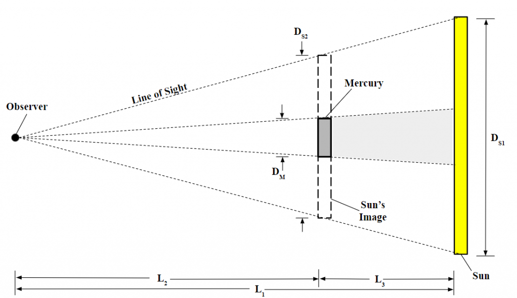
The figure shows the observer, the Sun, Mercury, and the Sun’s apparent image at the same distance as Mercury. The diagram has the following variables:
DS1 = Diameter of Sun
DS2 = Diameter of Sun’s Image
DM = Diameter of Mercury
L1 = Distance from Earth to Sun
L2 = Distance from Earth to Mercury
L3 = Distance from Mercury to Sun
Because both Mercury and the Sun are spheres, the following diagram is geometrically equivalent.
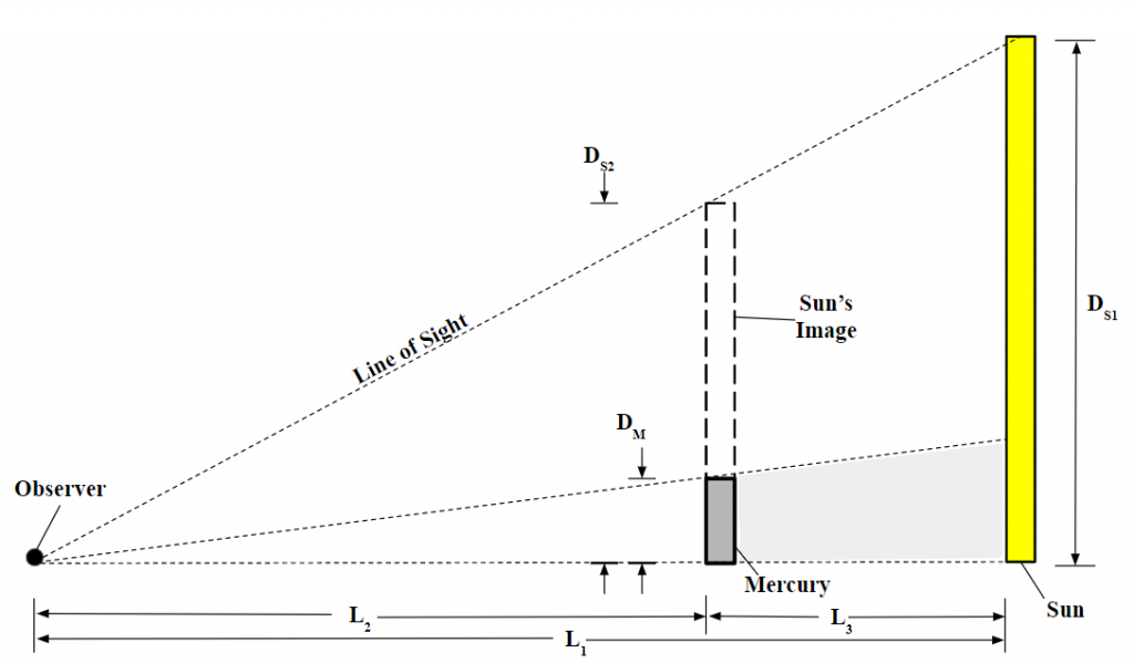
This diagram is necessary because it enables the law of similar triangles to be performed in order to establish relationships between various distances and diameters. The values of L1 and L2 for November 11, 2019 were obtained through a solar system simulator [10], and are as follows:
L1 = 0.990 AU
L2 = 0.675 AU
L3 can be defined as the difference between L1 and L2 and was determined to be as follows:
L3 = L1 – L2
L3 = (0.990 AU) – (0.675 AU)
L3 = 0.315 AU
The photosphere is the outermost layer of the Sun that is visible to the naked eye. According to the Stanford Solar Center, it has an approximate diameter of 1.391×10⁹ m [13]. This is the value for DS1.
DS1 = 1.391×10⁹ m
Now that L1, L2, and DS1 are known values, the law of similar triangles can be applied to Figure 3 in order to solve for DS2.
(DS1 / L1) = (DS2 / L2)
DS2 = (DS1 × L2) / L1
DS2 = [(1.391×10⁹ m) × (0.675 AU)] / (0.990 AU)
DS2 = 9.4841×10⁸ m
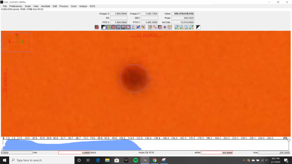
The ratio of DS2 to DM was then analyzed using AstroImageJ. The diameter of the Sun was measured to be 2908 pixels as seen in Figures 4 and 5. The diameter of Mercury was measured to be 15 pixels as seen in Figures 6 and 7.
The ratio of DS2 to DM was determined as the following:
(DS2) / (DM) = (2908 pixels) / (15 pixels)
(DS2) / (DM) = 193.87
Subsequently, the value of DS2 can be substituted in, and DM can be solved for as following:
(DS2) / (DM) = 193.87
DM = (DS2) / (193.87)
DM = (9.4841×10⁸ m) / (193.87)
DM = 4.8920×10⁶ m
The diameter of Mercury was calculated to be 4892 km. NASA’s measurement describes Mercury with a diameter of 4879 km [7]. This is a percent error of 0.27% for this calculation.
Angular Separation of Mercury and the Sun
The angular separation of Mercury and the Sun was calculated at the point when Mercury was at the midpoint of its transit. NASA’s Catalog of Transits of Mercury lists the start of the transit as 12:35 UTC and puts the end of the transit at 18:04 UTC [2]. This puts the midpoint of the transit at 10:20 EST. Image DSC_3314 was taken at 10:21 EST and was used for the calculation of angular separation.
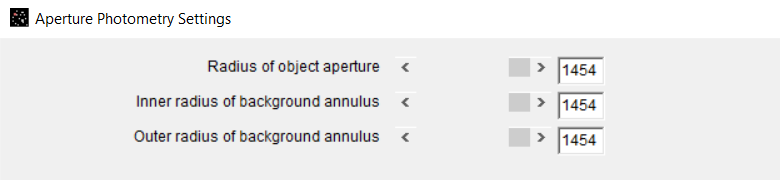
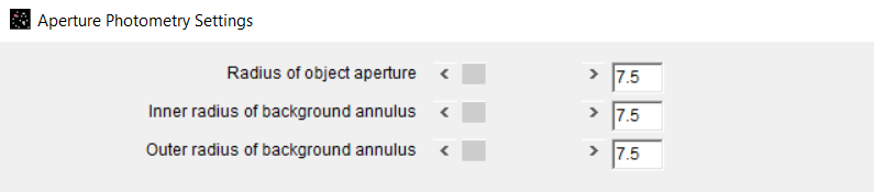
AstroImageJ was used to superimpose two concentric rings onto this image using aperture controls. The first ring was the exact size of the Sun’s disk and outlined the Sun’s border. The second ring, having the same center point as the first ring, had a radius such that the ring intersected the midpoint of Mercury.
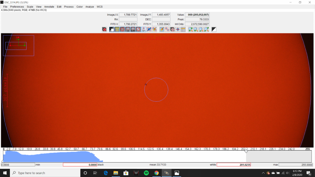
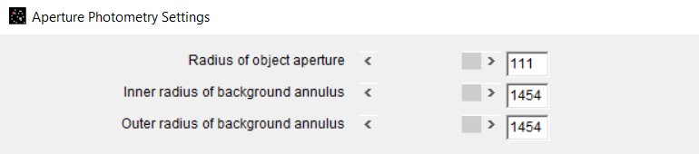
Because the rings are concentric, both rings were centered at the Sun’s midpoint. This means that the radius of the inner ring is the distance between the midpoint of the Sun and the midpoint of Mercury. If the diameter of the Sun’s disk was measured to be twice the radius, or 2908 pixels, and the separation of the midpoints of the two bodies was measured to be 111 pixels, the ratio of these distances can be represented as the following:
Angular Separation Ratio = (111) / (2908)
Angular Separation Ratio = 0.03817
This means that the angular separation of Mercury and the Sun is 3.817% of the angular diameter of the Sun. The angular diameter of the Sun can be found using the following equation:
[(2) × (π) × (L1)] / DS1 = (360 degrees) / DA
DA = Angular Diameter of Sun
Substituting the previous values for DS1 and L1, the following value is obtained for DA.
DA = 0.538 degrees
Multiplying this value by the Angular Separation Ratio obtained earlier, the following value is obtained for AM:
AM = (DA) × (0.03817)
AM = (0.538) × (0.03817)
AM = 0.0205 degrees
AM = Angular Separation of Mercury and Sun
The angular separation of Mercury and the Sun was calculated to be 0.0205 degrees, or 1.23 arcminutes at the midpoint of Mercury’s transit.
Inclination of Mercury’s Orbit
The angle of Mercury’s orbital location with respect to Earth’s orbital plane was calculated. The following diagram is a two-dimensional representation.
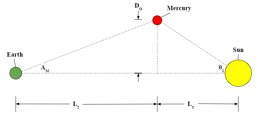
The following are new variables used:
θ2 = Mercury’s angular separation from Earth’s orbital plane
DO = Distance from Mercury to Earth’s orbital plane
Because L2, L3, and AM are known, DO, and subsequently, θ2 can be calculated. The calculation for DO is as follows:
tan(AM) = (DO) / (L2)
(L2) × tan(AM) = DO
(0.675 AU) × tan(0.0205 degrees) = DO
DO = 5.3535 × 10⁷ m
Now that DO is known, θ2 can be solved for as follows:
tan(θ2) = (DO) / (L3)
θ2 = tan-1[(DO) / (L3)]
θ2 = tan-1[(5.3535 × 10⁷ m) / (0.315 AU)]
θ2 = 0.06508 degrees
The angle of Mercury’s orbital location with respect to Earth’s orbital plane was calculated to be 0.06508 degrees. This value is different than the inclination of Mercury’s orbit. It was determined that not enough information was gathered during the transit to determine the inclination of Mercury’s orbit. In order to calculate the inclination of Mercury’s orbit, the value used for DO must be the maximum distance between Mercury and Earth’s orbital plane. Because Mercury was not at this point during the transit, the maximum distance cannot be determined from the data gathered during the transit. NASA’s calculations put the inclination of Mercury’s orbit at 7.01 degrees, significantly more than the 0.065 degrees observed [8]. This large difference is one of the reasons that transits of Mercury are rare. A significant amount of the times that the orbits of Earth and Mercury pass each other, the angle of Mercury’s orbital location with respect to Earth’s orbital plane is greater than the small angle necessary for a transit to be observable.
Historical Calculation Using Kepler’s Laws
In the 17th century, Johannes Kepler created a series of astronomical laws that govern orbiting bodies. He used these laws to establish relationships between the orbital distances of the planets in our solar system. Because of these laws, astronomers knew that the distance between Mercury and the Sun was about 35% to 40% of the distance between Earth and the Sun, but nobody knew how far either of these distances were [15]. It wasn’t until 1716 that astronomer Edmond Halley theorized a way to use the transit of Venus to calculate the exact distance from Earth to the Sun, also called an Astronomical Unit. He did this using the orbital laws that Kepler had created over 100 years beforehand. Unfortunately, by the next time Venus transited in 1769, both Kepler and Halley were dead. Fortunately, Halley’s theories were known well enough that many astronomers used the 1769 transit of Venus to calculate the exact value of an AU. Using these calculations, the distance from Earth to the Sun was calculated to be around 95 million miles, about 2% different from the 92.96 million miles that defines an AU today. Halley’s idea to calculate the distance from Earth to the Sun was based on the principle of parallax, the shift in apparent position that results from viewing an object from a different location. The following diagram shows the effect parallax has on planetary transits.
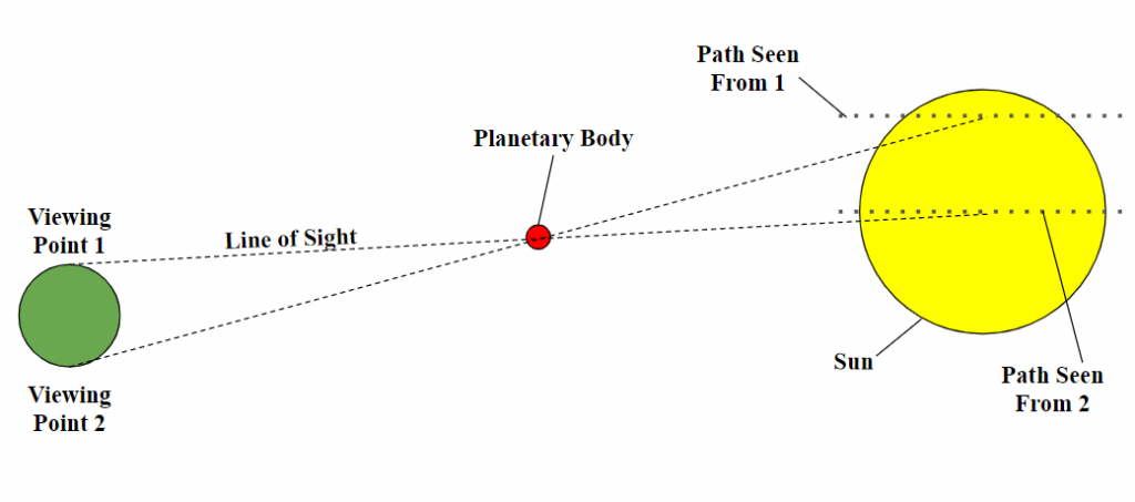
As exaggerated by the diagram, someone viewing the transit from viewing point 1 would observe the planet transiting across the lower portion of the Sun, while someone viewing the transit from viewing point 2 would observe the opposite. The transit, as observed from these 2 points, would also begin and end at different times, and the length of the transit would be observed to be shorter from viewing point 2. It is the difference in these times that allowed astronomers to calculate the distance from the Earth to the Sun. This same principle can be applied to the transit of Mercury and the value of an AU could be calculated. This was not done with this data because it requires the transit to be observed from two different viewing points a significant distance apart from one another.
Light Curve
Analyzing the light curve produced by planets transiting stars that are outside of our solar systems is a common method for determining the characteristics and existence of these exoplanets. This type of analysis was attempted with the data obtained during this solar transit. Using AstroImageJ, the average brightness for all pixels included in the disk of the sun was analyzed and plotted for a series of 200 images taken during the egress of Mercury. In other words, the amount of light reaching the Earth from the Sun was measured to see if there was a difference between when Mercury was in between Earth and the Sun, and when it was out of the way. In theory, the light curve should be consistent as Mercury transits, but rise slightly and steadily as Mercury leaves the disk of the Sun. In the data analyzed, this begins around the 120th image analyzed, or slice, and finishes around the 185th image analyzed. During this increment, the light curve should be increasing slowly and consistently. Before and after this increment, the light curve should remain constant.
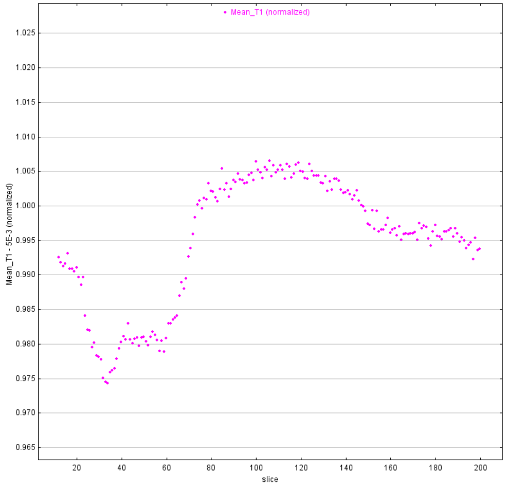
As seen in Figure 13, the results that were obtained are not consistent with the results that were expected. The variations and unpredictability of the curve are most likely due to changing atmospheric conditions and inconsistencies in cloud coverage, not because of the change in the amount of light obstructed by Mercury. These results dictate that this method is ineffective at determining characteristics of Mercury using the software programs and imaging hardware that were used for this observation.
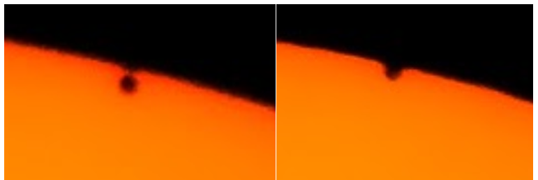
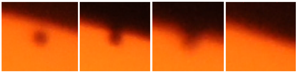
Black Drop Effect
The Black Drop Effect is an optical phenomenon that occurs when Mercury or Venus transit across the Sun. It is characterized by the teardrop shape that the planet’s disk makes as it makes contact with the edge of the Sun. The Black Drop Effect has historically caused confusion and frustration among astronomers seeking to make precise measurements about the solar system [14]. The exact cause is unknown, but it is probably a result of multiple factors including distortion of the light from Earth’s atmosphere, and a blurred effect from the point spread function of telescopes. Images DSC_3679, DSC_3718, DSC_3663, DSC_3709, DSC_3720, and DSC_3804 show a progression of Mercury’s egress that partially displays the black drop effect.
Limb Darkening
Limb Darkening is an optical effect where the brightness of the disk of the Sun gradually decreases from the center to the edges. Limb darkening occurs because the solar atmosphere increases in temperature with depth [15]. In the center of the solar ring, the observer sees the thickest and deepest layer of atmosphere that produces the most light. Towards the Sun’s limbs, only the upper layers of the solar atmosphere can be seen, and less light reaches the observer.
There are multiple mathematical models used today to describe the intensity of light as a function of the angle of incidence of the line of sight. These mathematical models help astrophysicists predict information about the Sun’s atmosphere and composition.
Conclusion
In conclusion, the purpose of this project was to investigate how much knowledge could be gained about the solar system using the imaging hardware and software available. The diameter of Mercury was calculated, the angular separation of Mercury and the Sun was calculated, Mercury’s orbital angular inclination was calculated, a historical calculation was repeated, the light curve of the transit was obtained and analyzed, the black drop effect was observed, and the limb darkening effects were analyzed. This was all done using equipment and software available to Howard Community College. The undergraduate research program at HCC has enabled students to complete projects like this, and many others. In the future, similar and more advanced projects for students can be envisioned, giving students the opportunity to learn how to conduct research, and further progress scientific knowledge.
Acknowledgements
I would like to thank Kenny Diaz, whose personal observing equipment was used during the transit operation.
Contacts: gbunyard7@gmail.com, bdiamond@howardcc.edu
References
[1] “AstroImageJ,” AstroImageJ (AIJ) – ImageJ for Astronomy. [Online]. Available: https://www.astro.louisville.edu/software/astroimagej/. [Accessed: 17-Mar-2020].
[2] “Catalog of Transits of Mercury,” NASA. [Online]. Available: https://eclipse.gsfc.nasa.gov/transit/catalog/MercuryCatalog.html. [Accessed: 17-Mar-2020].
[3] F. Espenak, “2019 Transit of Mercury,” EclipseWise. [Online]. Available: http://www.eclipsewise.com/oh/tm2019.html. [Accessed: 17-Mar-2020].
[4] “Helios Solar Glass® Filters,” Seymour Solar LLC. [Online]. Available: https://seymoursolar.com/product/helios-solar-glass-filters/. [Accessed: 17-Mar-2020].
[5] H. Neckel and D. Labs, “Solar limb darkening 1986–1990 (λλ303 to 1099 nm),” Solar Physics, vol. 153, no. 1-2, pp. 91–114, 1994.
[6] “November 11–12, 2019 Mercury Transit,” timeanddate.com. [Online]. Available: https://www.timeanddate.com/eclipse/transit/2019-november-11. [Accessed: 17-Mar-2020].
[7] “Overview,” NASA, 28-Jan-2020. [Online]. Available: https://solarsystem.nasa.gov/planets/mercury/overview/. [Accessed: 17-Mar-2020].
[8] “Planetary Fact Sheet,” NASA. [Online]. Available: https://nssdc.gsfc.nasa.gov/planetary/factsheet/. [Accessed: 17-Mar-2020].
[9] “Size of the sun (article),” Khan Academy. [Online]. Available: https://www.khanacademy.org/partner-content/nasa/measuringuniverse/measure-the-solarsystem/a/size-of-the-sun. [Accessed: 17-Mar-2020].
[8] “Solar Model,” Solar System Live. [Online]. Available: https://www.fourmilab.ch/cgi-bin/Solar. [Accessed: 17-Mar-2020].
[9] G. StefanssonI and Pennsylvania State University, “AstroImageJ: A Simple and Powerful Tool for Astronomical Image Analysis and Precise Photometry,” astrobites, 15-Apr-2016. [Online]. Available: https://astrobites.org/2016/04/15/astroimagej-a-simple-and-powerful-tool-for-astronomical-image-analysis-and-precise-photometry/. [Accessed: 17-Mar-2020].
[10] The Editors of Encyclopaedia Britannica, “Limb darkening,” Encyclopædia Britannica, 20-Apr-2018. [Online]. Available: https://www.britannica.com/science/limb-darkening. [Accessed: 17-Mar-2020].
[11] “The Sun’s Vital Statistics,” Stanford Solar Center. [Online]. Available: http://solar-center.stanford.edu/vitalstats.html. [Accessed: 17-Mar-2020].
[12] “What is the Black-Drop Effect?,” Sky & Telescope, 26-Feb-2020. [Online]. Available: https://www.skyandtelescope.com/astronomy-news/what-is-the-black-dropeffect/. [Accessed: 17-Mar-2020].
[13] “Why Is It Important?,” Exploratorium. [Online]. Available: https://www.exploratorium.edu/venus/question4.html. [Accessed: 17-Mar-2020].
