Up and Away! Rebound Height and Energy Changes in a System of Collisions

JRIP Editorial Team

Up and Away! Rebound Height and Energy Changes in a System of Collisions

Zainah Wadi, Howard Community College
Morin French, Howard Community College
Nian Liu, Howard Community College
Mentored by: Alex M. Barr, Ph.D.

Abstract

We investigate a vertical collision of two stacked balls experimentally, algebraically, and numerically to determine how various factors influence the rebound height. We calculated the predicted rebound height for both an elastic collision as well as an inelastic collision where the percent of kinetic energy each ball loses was determined experimentally using Tracker video analysis to analyze the stacked ball drop. We also modeled the experiment numerically in GlowScript where the upper ball is modeled as a system of two masses connected by a spring. The oscillations in the two-mass system act as a limited representation of the mechanical energy of the tennis ball converting to internal energy during each collision.

Introduction

Oftentimes simple experiments can be conducted to reveal explanations to seemingly complex phenomena. Supernovas and gravitational assist orbits can be better understood by investigating conservation of energy and momentum in a stacked ball drop. A stacked ball drop is when two or more balls are stacked vertically and dropped, and the top ball (ball 1) has a rebound height greater than the initial drop height. In a scenario with two balls being dropped, the bottom ball’s (ball 2) collision with the floor changes its velocity from the downwards direction to upwards. Ball 1 is traveling downwards when it collides with ball 2 which is traveling upwards. In this collision, ball 2 transfers energy to ball 1, changing the direction and magnitude of the velocity of ball 1. Using equations of conservation of energy and momentum, we can calculate the rebound height.

This phenomenon relates to a supernova because the star has a dense core that transfers a shock wave of energy outward. The transfer of energy from the dense core outward to the less dense layers causes the less dense layers to accelerate, resulting in a large velocity [1]. Collisions are typically thought of as two or more objects making physical contact; however, the same principle can be applied to a spacecraft utilizing a gravity assist maneuver. When a spacecraft enters a planet’s gravitational field some of the planet’s orbital energy can be transferred to the spacecraft, increasing the velocity of said spacecraft [2]. The sum of kinetic energy of the planet and spacecraft is preserved, however, so the interaction can be considered an elastic collision.

Mellen explored the behavior of a stacked collision that uses 7 different balls and compared the experimental data to his projected theoretical outcomes [2]. To perform the experiment with such a high number of balls he built a custom ball aligner, which he describes in detail in his paper. To determine the theoretical rebound height, Mellen used conservation of momentum with the coefficient of restitution. The coefficient of restitution is the ratio of relative velocity after the collision to relative velocity before the collision. The kinetic energy lost from each object is not distinguished, rather, the coefficient of restitution is accounting for the kinetic energy lost in the system as a whole.

Alternatively, we examined the kinetic energy lost from each ball as a separate entity. We use this along with the equations of conservation of momentum and energy to calculate theoretical rebound heights. We also modeled the collision in Glowscript to show how the kinetic energy is transformed into other forms of energy, a process we will discuss later in the paper.

Algebraic Solutions

To understand how a larger rebound height occurs, we begin by examining the scenario as an elastic collision.

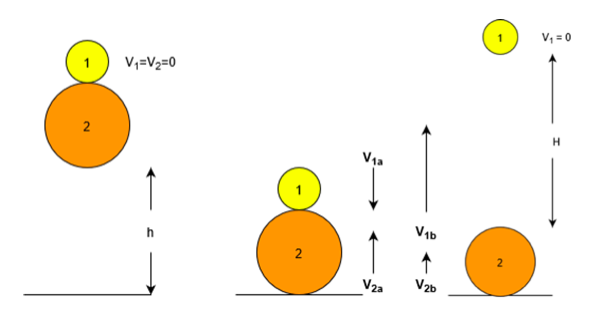
**Figure 1:** The image to the left is ball 1 and ball 2 at the initial height (h). The center image depicts the direction of velocity for each object at moment a (before the collision) and b (after the collision). The image to the right depicts the rebound height (H) of ball 1.

Figure 1 depicts the stacked ball drop, collision, and rebound of ball 1. Balls 1 and 2 both fall a distance of h. Ball 2 collides with the floor, changing direction before the collision and ball 1 rebounds to a height H measured from the point of collision. The equations for conservation of kinetic energy and momentum can be manipulated to find the rebound velocity of ball 1.

$\frac{1}{2}m_1v_{1a}^2+\frac{1}{2}m_2v_{2a}^2 = \frac{1}{2}m_1v_{1b}^2+\frac{1}{2}m_2v_{2b}^2$ (1)

$m_1v_{1a}^2+m_2v_{2a}^2 = m_1v_{1b}^2+m_2v_{2b}^2$ (2)

We can simplify the equations by canceling out the ½’s in equation (1) and introducing the mass ratio

$r = \frac{m_1}{m_2}$ (3)

This results in the equation:

$rv_{1a}^2+v_{2a}^2 = rv_{1b}^2+v_{2b}^2$ (4)

To determine the velocity of ball 1 and 2, we know that the gravitational potential energy at the starting position is equal to the kinetic energy the instant right before the ball collides with the ground. This relationship can be rewritten to obtain velocity.

$mgh = \frac{1}{2}mv^2 \rightarrow v = \pm \sqrt{2gh}$ (5)

The sign of velocity is determined by the direction before the collision, down is negative and up is positive. This results in $v_{2a}=+\sqrt{2gh}$ and $v_{1a}=-\sqrt{2gh}$ . With the velocities before the collisions defined, there are now two unknowns and two equations. Equations (4) and (5) can be combined to have the single unknown $v_{1b}$ .

$rv_{1a}^2 + v_{2a}^2 = rv_{1b}^2 + (r(v_{1a}-v_{1b})+v_{2a})^2$ (6)

To determine the ratio of the rebound height with respect to the original height, $v_{1b}$ is written

$v_{1b} = x|v_{1a}| = x\sqrt{2gh}$ (7)

Using kinetic energy and gravitational potential energy, H can be solved for as

$\frac{1}{2}mv_{1b}^2 = mgH \rightarrow \frac{1}{2}m(x\sqrt{2gh})^2 = mgH \rightarrow x^2h = H$ (8)

In equation (8), x²is the ratio of the rebound height to the initial height. Equation (6), however, is only true in an elastic collision. In the real-world there is a percentage of kinetic energy lost during the collisions of ball 2 with the ground and ball 1 with ball 2. The energy ball 1 loses can be accounted for by multiplying the pre-collision kinetic energy by a factor of $\alpha_1$ .

$\alpha_1rv_{1a}^2+v_{2a}^2 = rv_{1b}^2+(r(v_{1a}-v_{1b})+v_{2a})^2$ (9)

When ball 2 collides with the ground, the energy lost can be accounted for in the value of $v_{2a}$ .

$v_{2a} = \sqrt{\alpha_2 2gh}$ (10)

$\alpha_2$ signifies the percentage of kinetic energy remaining after the collision. Equations (9) and (10) can now be used to solve for the rebound velocity of ball 1 in an elastic collision ( $\alpha_1 = \alpha_2 = 1$ ) or in a collision where each ball loses a specified percentage of kinetic energy.

Experimental Results

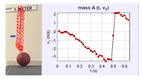
To determine the kinetic energy lost from the collision between ball 1 and 2, Tracker [4] was used to analyze a video of the collision between a tennis ball (ball 1) and basketball (ball 2) frame by frame to measure the velocity before and after the collision.

**Figure 2**: (Left) Tennis ball’s position for a sequence of video frames. (Right) Vertical velocity vs. time graph for the tennis ball bouncing off a stationary basketball. The vertical velocity of the tennis ball before the collision is -3.229 m/s and the vertical velocity after the collision is 2.116 m/s.

The percent kinetic energy remaining can be found by using the tennis ball velocity before and after it collides with the basketball.

$\frac{v_f^2}{v_i^2}\times 100 = \%~kinetic~energy~remaining$ (11)

$\frac{|2.116~m/s|^2}{|-3.229~m/s|^2}\times 100 = 43\%$

This value is used as the $\alpha_1$ value in equation (9). This process is repeated for ball 2 bouncing off the floor and that value is recorded as $\alpha_2$ . These values were used to create three curves displaying the rebound ratio (H/h) with respect to the mass ratio (r); an elastic collision, a collision where only ball 1 experiences energy loss, and a collision where both ball 1 and ball 2 experience energy loss. The graph shows that as the r value approaches zero, the energy lost from the ball 2 has a greater impact on the rebound height than the energy loss of ball 1 alone. As r approaches one, the impact of the energy lost from the ball 2 decreases. This is plausible because momentum and energy are quantities calculated using mass and velocity. In this scenario, ball 1 and 2 have the same magnitude of velocity but different masses, therefore, the object with the greater mass is contributing more energy and momentum to the system. When r approaches zero, the mass of ball 1 is negligible compared to the mass of ball 2 resulting in a greater decrease in rebound height when accounting for the energy lost from ball 2. As r approaches 1, the difference in mass of ball 1 and ball 2 is decreasing until they become the same mass at r = 1 causing the energy lost from ball 1 and 2 to have equal impacts on the rebound height.

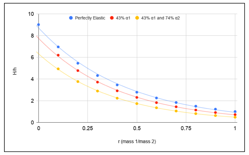
**Figure 3:** Rebound height ratio (H/h) vs. the mass ratio of ball 1 to ball 2 (r) for the three scenarios.

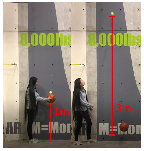
When comparing the algebraic solution and the experimental results, we begin by examining the mass ratio of the tennis ball to the basketball, which is approximately 0.1. Figure 3 illustrates that in a collision where r = 0.1, $\alpha_1=43\%$ and $\alpha_2=74\%$ the final height of the tennis ball when the system is dropped from 1 meter should be approximately 5 meters. Our experimental data does not support this claim. Figure 4 shows that the tennis ball only reaches 3 meters.

**Figure 4:** Experimental results for the stacked ball drop. (Left) The system at rest at the initial drop height. (Right) The tennis ball at its maximum rebound height.

Numerical Model

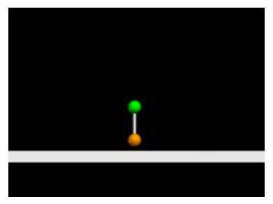
In the experiment, the mechanical energy of the tennis ball–basketball system decreases during the collision. Our algebraic solutions account for a percentage energy reduction but are unable to model the mechanism or possible forms to which the mechanical energy may be converted. To explore these questions, we modeled the collision in Glowscript, an adaptation of VPython, where we explicitly calculate the forces exerted on each ball at each moment. The change in forms of energy of the tennis ball was our primary focus; assuming that a significant amount of the mechanical energy was converted to internal energy, we modeled the tennis ball as two masses connected by a spring. The compression of the spring represents the deformation of the tennis ball during the collision. To investigate how the stiffness of that spring impacts the amount of energy transformed from mechanical to internal, we chose various spring constants and ran separate iterations of the program for each spring constant.

The lower ball was a necessary component of the simulation, but we were less interested in its behavior. Therefore, it was modeled as a single mass with an associated spring constant, whose primary purpose was to emulate the impact of the basketball colliding with the floor.

**Figure 5:** The tennis ball modeled as 2 spheres connected by a spring.

The greater the spring constant k, the greater the “stiffness” of the spring. A greater k constant should yield a more elastic collision, because stiffer springs do not easily transfer energy. A lack of energy transfer or transformation leaves no opportunity for energy loss, so the collision would conserve mechanical energy; ergo it would be an elastic collision. Taking the average forward deformation of a tennis ball (the amount it “squishes” upon impact), we calculated a minimum possible k constant for an elastic collision using conservation of energy [5]. By relating the gravitational potential energy before the drop to the elastic potential energy in the instant the tennis ball stops during the collision, we find our minimum k:

$GPE = EPE \rightarrow mgh = \frac{1}{2}k(\Delta L)^2$ (12)

$(0.059kg)(9.8\frac{m}{s^2})(1m) = \frac{1}{2}k(0.0065cm)^2 \rightarrow k=27.370.4142\frac{N}{m}$

When our tennis ball and basketball are dropped from 1 meter and k = 27,370.4142 N/m we ought to see a significant rebound height. Instead we see a rebound of less than 1.5 times the initial drop height, despite what the algebraic results would suggest.

**Figure 6:** Graph showing the y-position of center of mass of the tennis ball. After the bounce the rebound height should be considerably greater than the initial drop height, but that is clearly not the case.

If we substitute lesser and lesser k constants into the Glowscript model the collision should become more inelastic. Just as a greater k constant meant a stiffer spring, a lesser k constant means a less stiff spring. Decreasing the stiffness of the spring allows more energy to be transferred to elastic potential as the spring compresses, which in turn means we cannot achieve an elastic collision. In our simulation, we struggled to work with such reduced k constants. We reduced k from ~27,000N/m to 270N/m to 2.7N/m to model increasing amounts of mechanical energy being converted to elastic potential energy. However, in a low k simulation with just the tennis ball we see the two mass halves exchange position, which is physically impossible. Returning to equation (13) for conservation of energy we see that if GPE = EPE at low k values we, in turn, get a large $\Delta L$ :

$(0.059kg)(9.8\frac{m}{s^2})(1m) = \frac{1}{2}(2.7\frac{N}{m})(\Delta L)^2$

$\Delta L=\sqrt{\frac{2mgh}{k}} \rightarrow \Delta L=0.65 m$

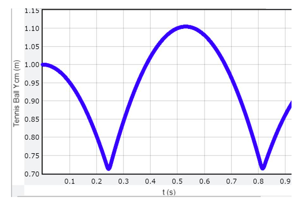
The average diameter of a tennis ball at rest is approximately 0.067m [5]. During the course of a collision, it is not possible for the tennis ball to stretch or compress beyond its initial length. Unfortunately, that is the behavior exhibited by the simulation. The smaller k constants were needed to produce a model that showed percent energy loss consistent with experimental data, but the behavior of the tennis ball at low k constants means that the model cannot be accurate. Although the intent of the numerical model was to create a simplified version of the vertical collision, the position and energy graphs from our simulations indicate that the model was too simplistic.

A fundamental problem underlying all other quirks of our numerical model is that it was built with the assumption that mass is distributed evenly across the tennis ball, and that the k remains constant across the ball and throughout an event such as a collision. This oversimplification fails to capture how the tennis ball would behave before, during, and after a collision. If one regards the tennis ball as a series of cross-sections, akin to Rod Cross’ analysis of the dynamics of a sphere, it becomes apparent that not all cross-sections have the same mass and that changes the stiffness of each section [6].

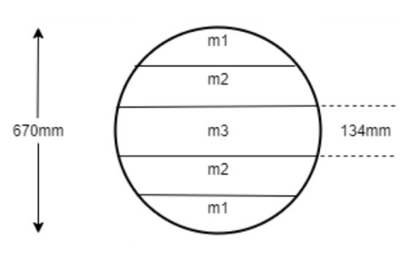
**Figure 7:** Illustration of cross sections of a tennis ball. Uneven mass distribution means m3 will have the greatest mass.

Using this more detailed model of a ball’s mass distribution, we can incorporate Young’s Modulus to predict the different k values for each cross section within the sphere:

$k = \frac{E*A}{w}$ (13)

where A = area of the cross-section, w = thickness of the cross-section, and E = Young’s Modulus, i.e. the force per unit surface along the bounce axis divided by the strain (proportional deformation). According to Cross, the end sections along the bounce axis will be considerably less stiff (smaller k values) because their cross-sectional area goes to zero at the edges.

With this representation of a spring constant, we find that k would stiffen as the sphere compresses on impact. The non-uniform distribution of mass also means that our system of only two masses and a spring will not be enough to accurately model the behavior of a ball during collision. Cross found some success modeling an elastic collision with a system of five masses and five springs, but even this would be insufficient to model an inelastic collision [6].

Conclusions

We investigated a vertical collision of two stacked balls algebraically to determine the rebound height of the top ball in both an elastic collision and where there is a percentage of energy loss in each ball. We gathered experimental data using Tracker and also modeled the experiment in Glowscript.

The algebraic model shows the significance the mass ratio holds for the rebound height. In order to have a greater transfer of energy to ball 1, it is imperative to have as small a mass ratio as possible. The algebraic model also demonstrates how energy loss from the more massive ball contributes greater to the energy loss of the whole system, decreasing the rebound height significantly. While conducting the experiment, it was quite difficult to get ball 1 and 2 to collide at a 90^oangle. The subtle inconsistency in drop angle could have an impact on the results for kinetic energy loss calculations from ball 1 and 2 as well as the rebound height of ball 1 during the experiment. The introduction of a ball aligner could decrease the effects of horizontal velocity.

To expand upon this project, the effects of drag can be incorporated into the calculation of the theoretical rebound height to determine if it is the cause of inconsistency between the experimental and theoretical rebound height.

Our numerical model proved too limited to accurately portray the stacked collision of a tennis ball and basketball. The tennis ball model was built utilizing the perspective of point particle physics employed in early physics classes; this led to such assumptions as that mass and spring constants would be uniform throughout each sphere. A more realistic approach could incorporate ideas more aligned with mechanics of materials, such as the application of Young’s Modulus as previously discussed.

Although our numerical model failed to meet our stated objective, we have stumbled across a potential exercise to help students make the leap from point particle physics to more advanced physics concepts. When tasked to create a simulation of a stacked ball drop, many early physics students would likely make the same erroneous assumptions we have made. Building (and subsequently troubleshooting) a model such as this, prompts students to identify for themselves the discrepancies and shortcomings of early physics lessons when discussing more complex concepts. In turn, this exercise creates an avenue through which students can begin to explore the shift in thinking required to move to higher-level physics and engineering courses.

Contacts: zainahwadi@gmail.com, morin.french@gmail.com, nian.jasmine@gmail.com, abarr@howardcc.edu

References

[1] Physics Girl. Stacked Ball Drop, (2015). Retrieved from

https://www.youtube.com/watch?v=2UHS883_P60.

[2] Huebner, J. S., & Smith, T. L. Multi‐ball collisions. The Physics Teacher,

30(1), 46–47 (1992). doi: 10.1119/1.2343467

[3] Mellen, W. R., Aligner for Elastic Collisions of Dropped Balls. The Physics

Teacher, 33 (1995).

[4] Tracker Video Analysis https://physlets.org/tracker/ (2019).

[5] 2018 ITF Ball Approval Procedures, (2019). Retrieved from

https://www.itftennis.com/media/2236/2020-itf-ball-approval-procedures.pdf.

[6] Cross, R., Differences between bouncing balls, springs, and rods. American Journal of Physics,
76, 908 (2008). https://aapt.scitation.org/doi/10.1119/1.2948778

License

Icon for the Creative Commons Attribution-NonCommercial-NoDerivatives 4.0 International License

Journal of Research in Progress Vol. 3 Copyright © 2020 by Howard Community College is licensed under a Creative Commons Attribution-NonCommercial-NoDerivatives 4.0 International License, except where otherwise noted.